Agriculture Water Use and Economic Value in the Great Salt Lake Basin
Utah’s Great Salt Lake
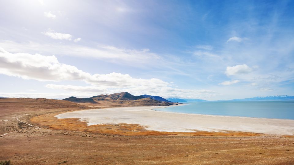
The Great Salt Lake (GSL) is the largest terminal saline lake in the western hemisphere and the eighth largest worldwide (Wurtsbaugh et al., 2016). Apart from the lake’s size, it adds value to Utah’s economy and environment by supporting industries, providing habitat for birds and other wildlife, increasing precipitation through the “lake effect,” and preventing dust storms that are harmful to human health (Null & Wurtsbaugh, 2020). Because GSL is a terminal lake (it has no outflow), it fluctuates in size year to year. Its size is based on a balance between the water evaporated from the lake and the water inflow into the lake. Historically, the inflow into the lake was primarily dependent upon precipitation in the GSL Basin (Figure 1). Generally, the lake has grown or shrunk in 5- to 30-year periods that coincide with droughts and wet periods (Brooks et al., 2021; Wurtsbaugh et al., 2016). For example, droughts in the 1960s were balanced by an unusually wet period in the 1980s (Null & Wurtsbaugh, 2020; Wine et al., 2019; Wurtsbaugh et al., 2017).
Purpose
This fact sheet provides information about with the following topics in the context of the Great Salt Lake and its basin:
- Great Salt Lake facts.
- Human effects on the size of the lake.
- Changes to population and land use.
- Agricultural water use.
- Agriculture and Utah’s economy.
- Foods produced by local agriculture.
Human Impact on the Great Salt Lake
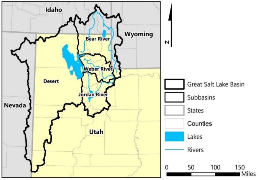
Sources: Natural Resources Conservation Service (NRCS, 2022); NRCS (2009); U.S. Census Bureau (2019); U.S. Geological Survey (USGS, 2019).
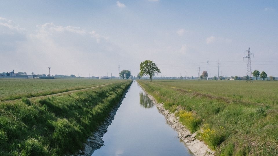
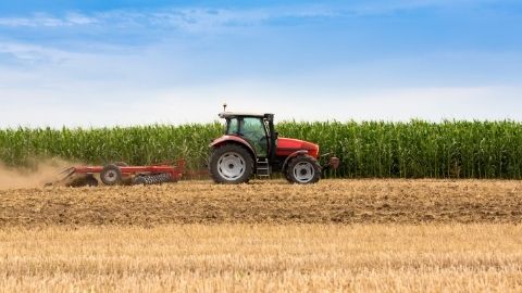
When settlers arrived 175 years ago, they undertook an ambitious project to tame the valleys around GSL and make the region productive for agriculture, industry, and a growing population. To do this, settlers diverted a portion of the water from streams and rivers that supply the GSL into extensive irrigation systems of canals and ditches.
It is estimated that nearly 45% of annual surface water flows from the three major rivers supplying the GSL is consumed by agriculture, municipal, and industrial uses (Wurtsbaugh et al., 2016). Even so, some additional water is delivered to the GSL basin from the Uinta basin using tunnels and aqueducts that are part of the Central Utah Project (CUP).
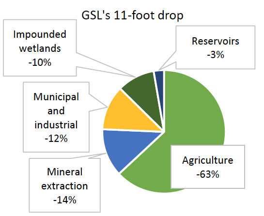
Overtime, human water use has caused an estimated loss of 11 feet to the GSL’s level and a 50% reduction of the lakebed area (Wurtsbaugh et al., 2016). Water depleted from the watershed due to human use is called consumptive use. Examples of sources of consumptive use in Utah include:
- Evapotranspiration from crops and ornamental plants.
- Steam from power plant cooling towers.
- Mineral extraction pond evaporation.
- Impounded wetlands and reservoir surface evaporation.
Consumptive water uses benefit Utah, and we can assign value to each of the examples above. Over 150 years, however, agriculture has consumed about five times the amount of water consumed by mineral extraction or municipal and industrial uses because agriculture has been in the GSL Basin the longest and was the most widespread land use (Wurtsbaugh et al., 2016). The consumptive use related to the 11 feet the lake has lost over 150 years is illustrated in Figure 2.
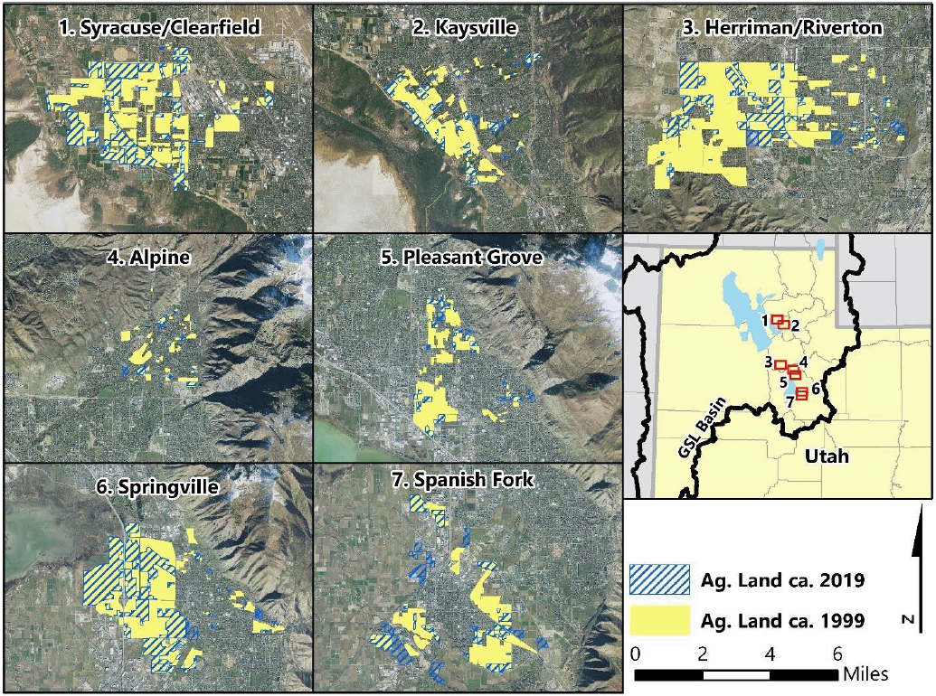
Historically, agriculture was the dominant land use in the Salt Lake Valley and, in turn, consumed most of the water, but today, much of the valley has been developed for housing. For example, agriculture’s share of water withdrawals in Salt Lake County is near 10% in 2015 compared to nearly 50% in 1985 (U.S. Geological Survey [USGS], 2023). Therefore, it is important to understand that water use changes as Utah grows.
Population Growth in Utah’s Great Salt Lake Basin
Utah’s population growth rate has surpassed the national average, and the high growth rate is expected to continue (Perlich et al., 2017). Much of the growth has occurred in the GSL Basin, specifically along the Wasatch Front, with population increasing by 1.33 million people between 1990 and 2020 (Table 1).
Over a similar period, 52,000 acres or 81 square miles of irrigated cropland were taken out of crop production (Figure 3), which is likely related to population growth. Our estimate compares the average irrigated acres from a period of moderate development (MD) (1982–1997) (Hassan et al., 2022) and a period of high development (HD) (2002–2017) (Hassan et al., 2022). The changes in irrigated acres for these periods are presented in Table 2.
Table 1.
Changes in Human Population Between 1990 and 2020 in the GSL Basin (×1,000)
| Basin | County | 19901 | 20202 | Difference |
|---|---|---|---|---|
| Bear River | Box Elder Cache Rich Basin total |
30.4 70.1 1.7 102.2 |
57.9 133.5 2.5 193.9 |
91% 90% 47% 90% |
| Jordan River | Salt Lake Tooele Utah Wasatch Basin total |
725.9 26.6 263.5 10.1 1,026.1 |
1,185.2 72.7 659.3 34.8 1,952.0 |
63% 173% 150% 245% 90% |
| Weber River | Davis Morgan Summit Weber Basin total |
187.9 5.5 15.5 158.3 367.2 |
362.2 12.2 42.3 262.2 679.3 |
93% 122% 173% 66% 85% |
| GSL Basin | 1,496 | 2,825 | 89% |
11990 population data are from the U.S. Census Bureau (1992).
22020 population data are from the U.S. Census Bureau, Population Division (2022).
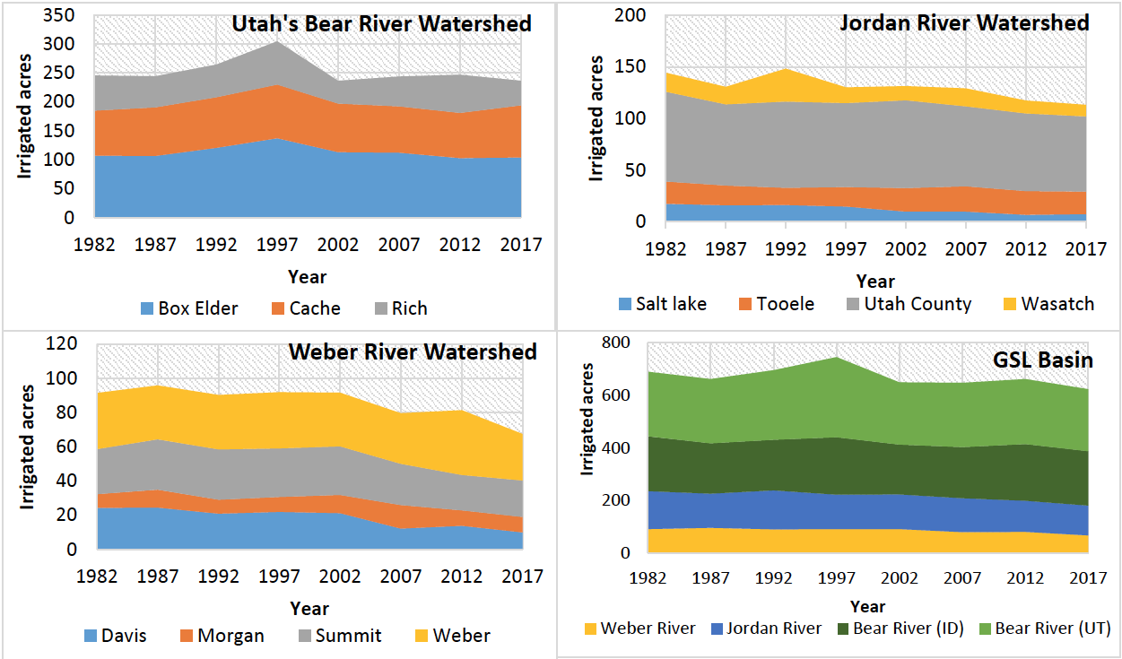
The Bear River Watershed (Bear River) supplies 58% of the inflow water to the GSL (Wurtsbaugh et al., 2016). It is also the least populated and least developed of the GSL’s tributary rivers. Between 1990 and 2020, the population increased by four people for each acre taken out of production. The Bear River also flows into Wyoming and Idaho in its course to the GSL. Because of this, out-of-state data are presented in Table 2.
The Jordan River Watershed (Jordan River) supplies 22% of the inflow water to the GSL (Wurtsbaugh et al., 2016). It has the largest human population of the three watersheds. Between 1990 and 2020, the population increased by 59 people for every acre taken out of production.
The Weber River Watershed (Weber River) contributes the least to the GSL at 15% of inflow (Wurtsbaugh et al., 2016). While not as populous as Jordan River, Davis and Weber counties are characterized by a growing suburban sprawl. Between 1990 and 2020, the population increased by 25 people per irrigated acre removed from production.
Between 2000 and 2020, municipalities on the Wasatch Front lost much of the cropland located near urban areas, such as Salt Lake City, Provo, and Ogden (Figure 4). The geography of the basin may be partially responsible for these land swaps. In the GSL Basin, nearly all the fresh surface water flows from the mountains east of the lakeshore, leaving a long narrow strip of arable land between the lake and the Wasatch Mountains.
Sources: Farm Service Agency (FSA, 2022); Natural Resources Conservation Service (NRCS, 2022); NRCS (2009); U.S. Census Bureau (2019); USGS (2019)
Table 2.
Change in Irrigated Acres Between 1982 and 2017, Estimated by the U.S. Department of Agriculture (USDA) (×1,000 acres)
|
|
|
|
---------------MD-------------- |
--------------HD------------- |
Difference MD to HD |
||||||
|
Basin |
|
Utah counties |
1982 |
1987 |
1992 |
1997 |
2002 |
2007 |
2012 |
2017 |
|
|
Bear River |
Box Elder |
107 |
106.7 |
120.6 |
137.1 |
112.1 |
102.9 |
103.8 |
108.0 |
-8% |
|
|
Cache |
78.1 |
83.8 |
87.5 |
93 |
80.2 |
78.1 |
90.1 |
83.1 |
-3% |
||
|
Rich |
60.5 |
54.0 |
56.4 |
74.6 |
51.8 |
66 |
42.4 |
49.9 |
-19% |
||
|
Watershed in Utah1 |
245.6 |
244.5 |
264.5 |
304.7 |
244.1 |
247.0 |
236.3 |
241.0 |
-9% |
||
|
Development period average in Utah |
264.8 |
241.0 |
|||||||||
|
|
---------------MD-------------- |
--------------HD------------- |
Difference MD to HD |
||||||||
|
Idaho counties |
1982 |
1987 |
1992 |
1997 |
2002 |
2007 |
2012 |
2017 |
|||
|
Bear Lake |
51.2 |
45.2 |
42.6 |
49.8 |
43.5 |
38.7 |
54.5 |
54.7 |
+1% |
||
|
Caribou |
70.3 |
66.0 |
70.2 |
80.8 |
67.2 |
68.3 |
66.0 |
61.1 |
-9% |
||
|
Franklin |
52.0 |
48.7 |
50.9 |
54.6 |
46.2 |
49.4 |
61.2 |
65.3 |
+8% |
||
|
Oneida |
34.6 |
31.1 |
28.9 |
33.4 |
32.5 |
38.3 |
34.1 |
25.7 |
-2% |
||
|
Watershed in Idaho1 |
208.1 |
191.0 |
192.6 |
218.6 |
189.4 |
194.7 |
215.8 |
206.8 |
0% |
||
|
Development period average in Idaho |
202.6 |
201.7 |
|||||||||
|
Difference in irrigated area in Idaho and Utah |
-24.7 |
||||||||||
|
Jordan River |
|
---------------MD-------------- |
--------------HD------------- |
Difference MD to HD |
|||||||
|
County |
1982 |
1987 |
1992 |
1997 |
2002 |
2007 |
2012 |
2017 |
|||
|
Salt Lake |
17.4 |
16.0 |
16.3 |
14.7 |
9.9 |
9.8 |
6.8 |
7.4 |
-47% |
||
|
Tooele |
21.6 |
19.0 |
16.5 |
18.9 |
22.8 |
24.5 |
23.0 |
21.9 |
21% |
||
|
Utah |
86.9 |
78.7 |
83.6 |
81.2 |
84.9 |
77.5 |
75.2 |
72.7 |
-6% |
||
|
Wasatch |
18.5 |
17.0 |
31.8 |
15.4 |
13.8 |
17.4 |
12.4 |
11.3 |
-34% |
||
|
Watershed1 |
144.4 |
130.7 |
148.2 |
130.2 |
131.4 |
129.2 |
117.4 |
113.3 |
-11% |
||
|
Development period average |
138.4 |
122.8 |
|||||||||
|
Difference in irrigated area |
-15.6 |
||||||||||
|
Weber River |
---------------MD-------------- |
--------------HD------------- |
Difference MD to HD |
||||||||
|
County |
1982 |
1987 |
1992 |
1997 |
2002 |
2007 |
2012 |
2017 |
|||
|
Davis |
24.3 |
24.5 |
21.0 |
21.9 |
21.3 |
12.2 |
13.8 |
10.0 |
-38% |
||
|
Morgan |
7.97 |
10.4 |
8.0 |
8.80 |
10.6 |
13.8 |
9.0 |
9.0 |
21% |
||
|
Summit |
26.4 |
29.4 |
29.4 |
28.4 |
28.3 |
24.0 |
20.8 |
21.3 |
-17% |
||
|
Weber |
32.8 |
31.5 |
31.8 |
32.7 |
31.4 |
29.6 |
37.7 |
27.1 |
-2% |
||
|
Watershed1 |
91.47 |
95.8 |
90.2 |
91.8 |
91.6 |
79.6 |
81.3 |
67.4 |
-13% |
||
|
Development period average |
92.3 |
80.0 |
|||||||||
|
Difference in irrigated area |
-12.3 |
||||||||||
|
GSL Basin |
---------------MD-------------- |
--------------HD------------- |
Difference MD to HD |
||||||||
|
1982 |
1987 |
1992 |
1997 |
2002 |
2007 |
2012 |
2017 |
||||
|
Watershed1 |
689.6 |
662.0 |
695.5 |
745.3 |
649.0 |
647.6 |
661.5 |
623.8 |
-8% |
||
|
Development period average |
698.1 |
645.5 |
|||||||||
|
Difference in irrigated area |
-51.7 |
||||||||||
1Irrigated acres data in 1987–2017 are from National Agricultural Statistics Service (NASS, 2019b).
Note.MD = moderate development and HD = high development
Agricultural Water Use in Utah’s Great Salt Lake Basin
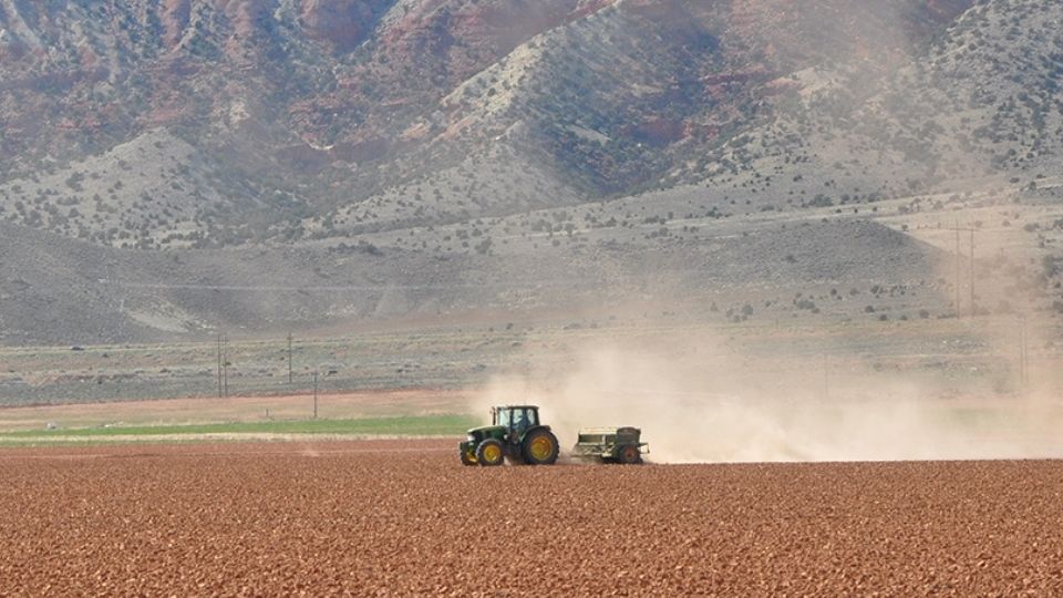
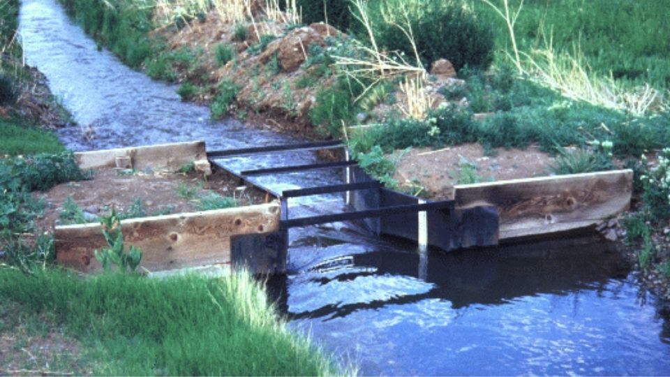
To understand agricultural water use, it is important to briefly explain water conveyance, irrigation methods, and the units for water delivery and consumption. Before water is applied to a field, it travels from its natural source to the field; this is conveyance.
Conveyance systems are used to transport water from a natural source to the water user. In Utah, conveyance usually begins as points in reservoirs or rivers where water is withdrawn from the source. The water is diverted at these points into a canal or pipeline by pumping or splitting the stream flow with human-made structures. Large canals and pipes (main channels) carry large volumes of water for several miles. Smaller ditches or pipelines (laterals) convey smaller water volumes from main channels to various sites or field ditches and pipelines that supply fields.
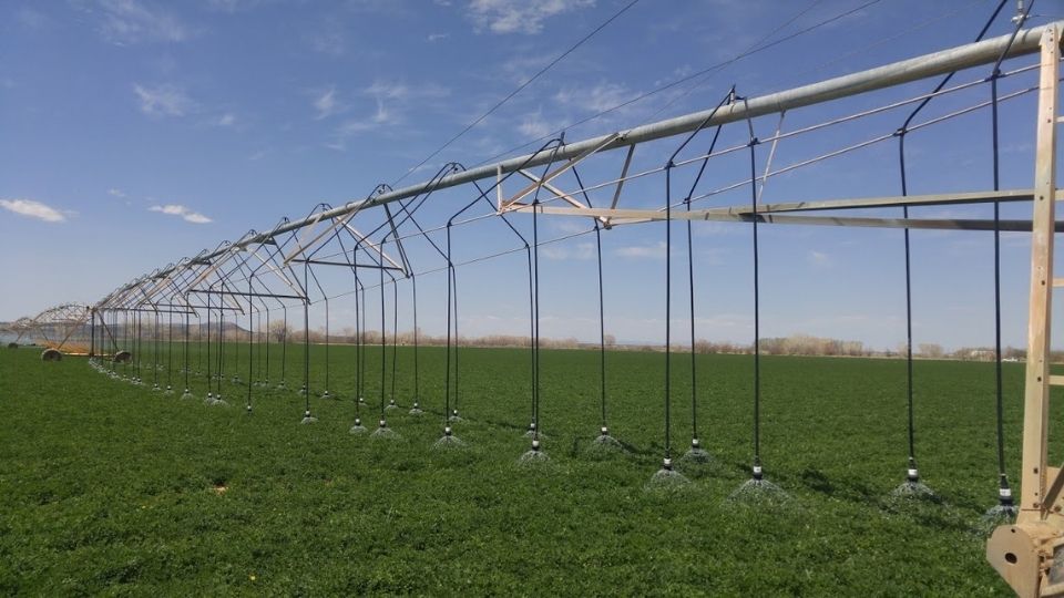
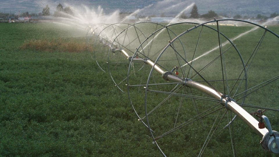
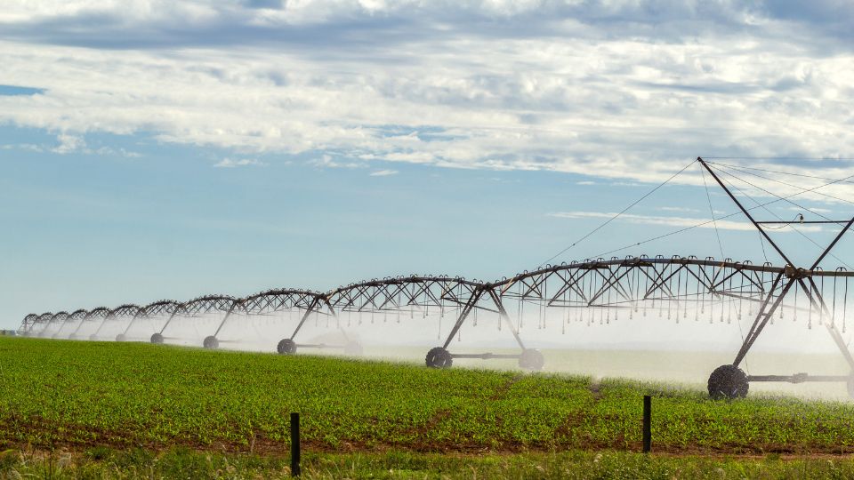
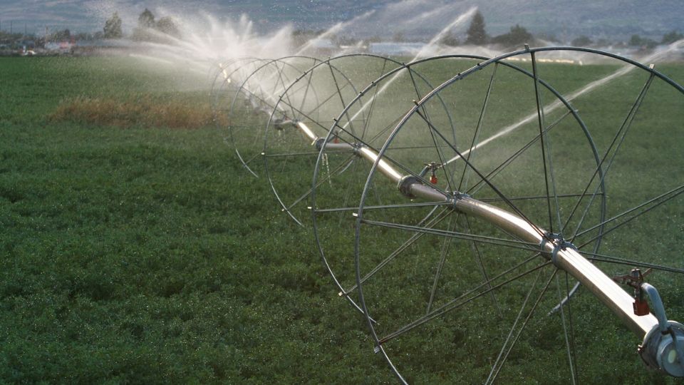
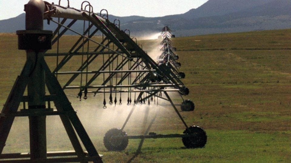
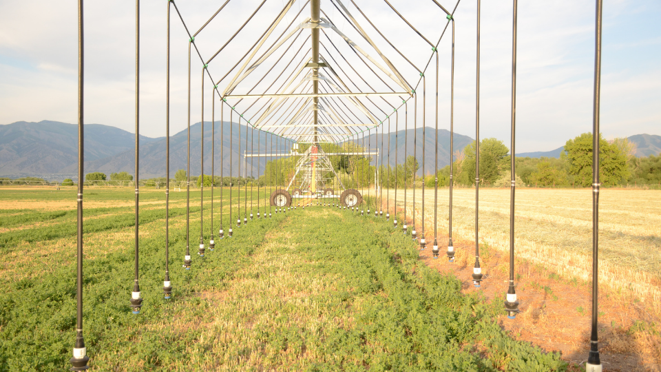
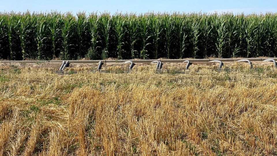
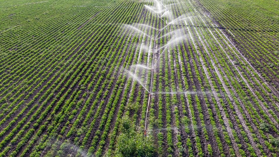
After the water reaches a field, several methods may be used to irrigate, including surface (wild flood, furrow, basin), sprinkler, and drip irrigation. Irrigation method efficiencies vary relative to both water available to the crop and consumptive use (Crookston et al., 2022).
Surface and drip irrigation methods tend to have less evaporation and wind drift losses than sprinklers. However, surface irrigation can have greater losses to runoff and deep percolation (drainage below plant roots) than drip and sprinklers. Moreover, deep percolation and runoff are not lost and are not consumptive use because the water will ultimately flow to a surface water body or to the groundwater table. In contrast, the watershed is less likely to recover losses from wind drift and evaporation. This results in relatively high consumptive inefficiencies for many sprinkler irrigation technologies. Each irrigation method has its own advantages and disadvantages, summarized in Table 3. Because of inefficiencies, each method requires a different amount of water to produce the same crop yield. The amount of water conveyed and used for irrigation is usually communicated as acre-feet or acre-inches rather than gallons because of the large volumes. A comparison of gallons, acre-feet, and other water volumes is found in Table 4. For reference, an acre-foot is equal to a football field flooded about 1 foot deep.
Table 3.
Efficiencies, Advantages, and Disadvantages of Various Irrigation Methods
| Method & application efficiency1 (%) | Advantages | Disadvantages |
|---|---|---|
| Surface (40%–90%) | Relatively low evaporative and wind drift losses and potentially low cost to implement. | Potentially nonuniform application across the field and large losses to deep percolation. Labor intensive. |
| Line-source sprinkler – wheel lines and hand lines (60%–80%) | Typically, more uniform water application than surface methods. | High potential for wind drift and evaporation. Equipment can be expensive. Can be labor intensive. |
| Center pivot sprinkler (80%–97%) | More options for increasing application precision. Greater automation than other methods. | Expensive to install. Varied potential for wind drift and evaporation. |
| Drip systems (≥90%) | Water is applied closer to the crop root zone, reducing evaporation and wind drift. Allows for soil surface barriers. Potentially automated. | Expensive and relatively high maintenance systems. Can have significant plastic waste. Relatively less ground water recharge. |
1Efficiency data are from Crookston, Peters, Yost, and Barker (2022).
Table 4.
Approximate Water Volumes and Conversions for Gallons and Acre-Feet
| Gallons | Water body1,2 | Acre-Feet |
|---|---|---|
| 325,851 | 1 | |
| 65,000 | Olympic size swimming pool | 0.2 |
| 7,500,000,000 | Lost Creek Reservoir | 23,000 |
| 16,000,000,000 | East Canyon Reservoir | 49,500 |
| 24,000,000,000 | Echo Reservoir | 74,000 |
| 36,000,000,000 | Pineview Reservoir | 110,000 |
| 49,000,000,000 | Deer Creek Reservoir | 150,000 |
| 100,000,000,000 | Jordanelle Reservoir | 314,000 |
| 280,000,000,000 | Utah Lake | 871,000 |
| 8,100,000,000,000 | Great Salt Lake (full at 4,208 ft) | 25,000,000 |
1Water capacities for reservoirs and Utah Lake are from Utah Division of Water Rights (2023).
2Water volume of GSL at 4,208 feet is from Mohammed and Tarboton (2011).
Utah agricultural irrigation withdrawals in the GSL Basin decreased by 588,000 acre-feet (30%) when comparing 1985 to 2015. Over the same period, agriculture’s share of total water withdrawals decreased by -25% in Utah. It’s unlikely the average annual withdrawal has decreased for the entire GSL Basin because of statewide irrigation trends (Barker et al., 2022). It is important to note that 1985 was an exceptionally wet year and 2015 was exceptionally dry. Because of this, natural flows and water stored in reservoirs would have decreased water availability in 2015 compared to 1985. Regardless of whether there has been an annual decrease in agricultural irrigation withdrawals, population growth, limited land area, irrigation optimization, and more efficient conveyance will likely result in a future downward trend of agricultural withdrawals in the GSL Basin.
In Bear River, agricultural irrigation withdrawals in Utah during 1985 and 2015 were very similar or slightly decreased (-1%) (Table 5). On a per acre basis, we estimate water allocations of 3.0 and 2.9 acre-feet in 1985 and 2015, respectively. Agriculture used 91% and 93% of the water withdrawn from the Bear River in 1985 and 2015, respectively (Table 6). An increase in Box Elder (+5) offset decreases in Cache (-6%) and Rich (-2%) counties.
In Jordan River, agricultural withdrawals decreased by 262,000 acre-feet (-39%) when comparing 1985 to 2015 (Table 5). On a per-acre basis, we estimate water allocations of 4.7 and 3.5 acre-feet in 1985 and 2015, respectively. The percentage of Jordan River water used by agriculture was 71% and 55% in 1985 and 2015, respectively (Table 6). The most significant decrease (-37%) was in Salt Lake County, the most populous in the GSL Basin.
In Weber River, agricultural withdrawals in 2015 were far less than in 1985, with an estimated decrease of 320,000 (-60%) (Table 5). On a per-acre basis, we estimate a water allocation of 5.9 and 2.7 acre-feet in 1985 and 2015, respectively. In the Weber River watershed, agricultural used 83% to 62% of withdrawn water in 1985 and 2015, respectively (Table 6). The most significant change (-45%) was Morgan County, the least populous county in Weber River.
Idaho counties with the most irrigated area apparently supplied by the Bear River were included in Table 5. USGS data shows there was a 452,000 acre-foot (+30%) increase in agricultural irrigation withdrawals in Idaho when comparing 1985 to 2015.
Table 5.
U.S. Geological Survey (USGS) Estimates of Annual Agricultural Irrigation Withdrawals for the GSL Basin in 1985 and 2015 (×1,000 acre-feet)
|
Basin |
Utah counties |
1985 |
2015 |
Difference |
|
Bear River |
Box Elder |
349 |
459 |
+32% |
|
Cache |
226 |
137 |
-39% |
|
|
Rich |
158 |
131 |
-17% |
|
|
Watershed in Utah1,2 |
733 |
727 |
-1% |
|
|
Difference in agricultural withdrawals in Utah |
-6 |
|||
|
Idaho counties |
1985 |
2015 |
Difference |
|
|
Bear Lake |
428 |
283 |
-34% |
|
|
Caribou |
331 |
502 |
+52% |
|
|
Franklin |
590 |
342 |
-42% |
|
|
Oneida |
150 |
824 |
+449% |
|
|
Watershed in Idaho1,2 |
1,499 |
1,951 |
+30% |
|
|
Difference agricultural withdrawals in Idaho |
+452 |
|||
|
Jordan River |
Utah counties |
1985 |
2015 |
Difference |
|
Salt Lake |
202 |
22 |
-89% |
|
|
Tooele |
68 |
93 |
+37% |
|
|
Utah |
305 |
260 |
-15% |
|
|
Wasatch |
97 |
35 |
-64% |
|
|
Watershed1 |
672 |
410 |
-39% |
|
|
Difference in agricultural withdrawals |
-262 |
|||
|
Weber River |
Utah counties |
1985 |
2015 |
Difference |
|
Davis |
112 |
45 |
-60% |
|
|
Morgan |
118 |
39 |
-67% |
|
|
Summit |
104 |
49 |
-53% |
|
|
Weber |
204 |
85 |
-58% |
|
|
Watershed1 |
538 |
218 |
-60% |
|
|
Difference in agricultural withdrawals |
-320 |
|||
|
GSL Basin |
|
1985 |
2015 |
Difference |
|
Basin total in Utah |
1,943 |
1,355 |
-30% |
|
|
GSL Basin total |
3,442 |
3,306 |
-4% |
|
|
Difference in agricultural withdrawals |
-136 |
|||
1Some golf courses may be included.
2Usage from other states is excluded.
Source: 1985 and 2015 data are from the USGS (2023).
Table 6.
USGS Estimates of Changes in Agricultural Withdrawals for the GSL Basin in 1985 and 2015 as a Percentage of Total Annual Withdrawals1
|
|
||||
|
Basin |
County |
1985 |
2015 |
Difference |
|
Bear River |
Box Elder |
91% |
96% |
+5% |
|
Cache |
86% |
80% |
-6% |
|
|
Rich |
100% |
98% |
-2% |
|
|
Watershed1 |
91% |
93% |
2% |
|
|
Jordan River |
County |
1985 |
2015 |
Difference |
|
Salt Lake |
49% |
12% |
-37% |
|
|
Tooele |
81% |
82% |
+1% |
|
|
Utah |
76% |
51% |
-25% |
|
|
Wasatch |
96% |
35% |
-61% |
|
|
Watershed1 |
71% |
55% |
-17% |
|
|
Weber River |
County |
1985 |
2015 |
Difference |
|
Davis |
72% |
56% |
-16% |
|
|
Morgan |
98% |
53% |
-45% |
|
|
Summit |
80% |
79% |
-1% |
|
|
Weber |
83% |
61% |
-22% |
|
|
Watershed1 |
83% |
62% |
-25% |
|
|
GSL Basin |
1985 |
2015 |
Difference |
|
|
Watershed in Utah1 |
82% |
77% |
-7% |
|
11985 and 2015 data are from USGS (2023).
It is difficult to accurately estimate consumptive water use, particularly at the scale of the GSL Basin. Here, a simple estimate was made based on the ratio of consumptive water use estimates to withdrawals reported by the USGS for 2015. In that year, agricultural irrigation consumptive use was estimated to be 66% of agricultural irrigation withdrawals in the 11 Utah counties included in this analysis (USGS, 2023). Based on a 66% estimate, agricultural consumptive use in the GSL Basin decreased by nearly 400,000 acre-feet when comparing 1985 to 2015 (Table 7). Although it doesn’t necessarily signal an annual decline, it suggests that there may be flexibility in annual water need given that hay yields were higher today on a per acre basis than yields in the 1980s (NASS, Mountain Region, Utah Field Office, 1991). This suggests that more research is needed to understand how production optimization may reduce average annual water need and increase flow to the GSL while maintaining agricultural productivity.
In Bear River, consumptive use from agricultural withdrawals in 1985 and 2015 shows little change. Consumptive use per acre was relatively constant at about 2.0 acre-feet per acre.
In Jordan River, consumptive use from agricultural withdrawals decreased by 179,000 acre-feet when comparing 1985 and 2015. Consumptive use per acre in the watershed was 3.2 and 2.4 acre-feet per acre in 1985 and 2015, respectively.
In Weber River, consumptive use from agricultural withdrawals decreased by 218,000 acre-feet when comparing 1985 and. Consumptive use per acre in the watershed was 4.0 and 1.8 acre-feet per acre for 1985 and 2015, respectively.
Table 7.
Calculated Consumptive1 Water Use as 66% of Agricultural Withdrawal in Utah’s GSL Basin ( ×1,000 acre-feet)
|
Basin |
County |
1985 |
2015 |
Difference |
||
|
Bear River |
Box Elder |
237.3 |
312.1 |
32% |
||
|
Cache |
153.7 |
93.2 |
-39% |
|||
|
Rich |
107.4 |
89.1 |
-17% |
|||
|
Watershed total |
498.4 |
494.4 |
-1% |
|||
|
30-year change in acre-feet |
-4 |
|||||
|
County |
1985 |
2015 |
Difference |
|||
|
Jordan River |
Salt Lake |
137.4 |
15 |
-89% |
||
|
Tooele |
46.2 |
63.2 |
37% |
|||
|
Utah |
207.4 |
176.8 |
-15% |
|||
|
Wasatch |
66.0 |
23.8 |
-64% |
|||
|
Watershed total |
457.0 |
278.8 |
-39% |
|||
|
30-year change in acre-feet |
-178.2 |
|||||
|
County |
1985 |
2015 |
Difference |
|||
|
Weber River |
Davis |
76.2 |
30.6 |
-60% |
||
|
Morgan |
80.2 |
26.5 |
-67% |
|||
|
Summit |
70.7 |
33.3 |
-53% |
|||
|
Weber |
138.7 |
57.8 |
-58% |
|||
|
Watershed total |
365.8 |
148.2 |
-60% |
|||
|
30-year change in acre-feet |
-218 |
|||||
|
GSL |
County |
1985 |
2015 |
Difference |
||
|
Basin total |
1,321.2 |
921.4 |
-30% |
|||
|
Difference in acre-feet |
-399.8 |
|||||
1Consumptive use calculation is 68% of data values from Tables 4, 7, and 10.
Source: 1985 and 2015 data from the USGS (2023).
Agriculture’s Economic Value in Utah’s GSL Basin
Maintaining GSL water elevations are important to preserve the $1.9 billion that the GSL contributes annually to Utah’s economy (Null & Wurtsbaugh, 2020). Irrigated agriculture in the GSL Basin is also important for the economy and environment of the watershed. Estimating the full economic contribution from agriculture on the GSL Basin is complex and beyond the scope of this fact sheet. A summary of a few items (cash receipts, farm input costs, and the GSL basin’s food commodity production) is included as some indication of the full economic contribution. Although irrigated agriculture does not comprise all the agricultural productivity in the GSL Basin, irrigation is an essential input that supports nearly all agriculture in the area; separating out the share of non-irrigated agriculture would be difficult, so non-irrigated data are also included.
Farm cash receipts are the payments received by the farmer from selling an agricultural commodity (Table 8). In 2017, farmers in the GSL counties received $740 million from these payments. That is an $881 million value in 2022 due to inflation. Cash receipts are the direct economic contributions from farmers but are not the total contribution. In a supply-driven approach, the full economic contribution would also include both the backward (supplies purchased) and forward linkages (food produced).
For example, between 2018 and 2022, U.S. dairy farmers usually sold their milk for $18–$25 per 100 pounds of milk or $1.54–$2.14 per gallon (Agricultural Marketing Service [AMS], 2022a). Over the same period, the price of milk per gallon in grocery stores was $3.27–$4.44 per gallon (AMS, 2018; AMS, 2022b). In this example, each gallon of milk had an added value of $1.73–$2.30 after farm cash receipts. Furthermore, a large portion of milk produced does not reach the grocery store as fluid milk; rather, it is processed into other value-added products (cheese, yogurt, ice cream, and butter), which may increase the agriculture economic contribution further.
Nationally, it has been estimated that farmers receive about 15 cents per dollar Americans spend on food (Dorfman, 2023). It is unknown if Dorfman’s estimate is true for Utah, but it’s reasonable to include value-added products or forward linkages in a supply-driven estimate like this. The bottom line is that cash receipts are not an accurate indicator of the total economic benefit from agriculture in the GSL Basin.
Farmer and rancher input costs (backward linkages) are substantial in the GSL Basin. To produce agricultural commodities, farmers and ranchers spend money on things such as labor, agrochemicals, seed, veterinarians, equipment, supplies, and a variety of other commodities. These costs are paid for each year using loans or cash from previous years. In 2017, farmers in the GSL Basin spent about $640 million, worth about $760 million in 2022 due to inflation (NASS, 2019a).
Following a supply-driven approach, it’s reasonable to assume that the economic contribution of agriculture is probably greater than $1.6 billion (direct receipts $881 million plus farm and ranch input costs) but likely less than $6.7 billion in the GSL Basin (total value of food from farm production).
Food commodities produced in the GSL basin are of significant value to the 2.8 million people in the basin, economic benefits aside. However, it is important to note that this fact sheet does not imply that food produced locally is consumed locally because food is imported and exported from Utah due to economic pressures and the structure of U.S. food supply chains. What is implied is the capacity of production for raw agricultural commodities.
Table 9 summarizes the amount of food produced in the GSL Basin for common items in most Utahns’ pantries and refrigerators. GSL Basin agriculture produces a significant amount of food considering the percentage of per capita production in the GSL Basin compared to U.S. per capita availability (Table 9).
Table 8.
Farm Cash Receipts1 in the Great Salt Lake Basin Counties in Utah
| County | Estimated 2022 Values2 |
|---|---|
| Utah | $238,714,000 |
| Box Elder | $201,760,000 |
| Cache | $193,657,000 |
| Weber | $58,837,000 |
| Tooele | $48,496,000 |
| Summit | $30,393,000 |
| Davis | $28,320,000 |
| Rich | $26,268,000 |
| Salt Lake | $23,682,000 |
| Morgan | $20,384,000 |
| Wasatch | $10,474,000 |
| Total | $880,985,000 |
1Cash receipts for 2017 are from NASS (2018).
2Dollars are adjusted for inflation using the consumer price index to represent the value of cash receipts in 2022.
Table 9.
Select Food Production and Per Capita Availability in Utah’s GSL Basin
| Food item | GSL Basin production (2017) | GSL Basin as percent of Utah’s production | Production per capita (GSL Basin) | GSL production as a percentage of estimated per capita need by GSL population1 |
|---|---|---|---|---|
| Wheat flour2 | 118 million lb | 72% | 71.4 lb | 55% |
| Milk (if no cheese) | 123 million gallons | 51% | 43.7 gallons | 280% |
| Cheese3 (if no milk) | 106 million lb | 51% | 37.6 lb | 96% |
| Beef4 (boneless) | 66.3 million lb | 23% | 23.5 lb | 42% |
| Eggs5 | 106 million dozen | 100% | 37.5 dozen | 115% |
| Peaches | 9.6 million lb | 91% | 3.4 lb | 73% |
| Apples | 10.6 million lb | 83% | 3.75 lb | 21% |
| Onions | 86 million lb | 98% | 30.5 lb | 138% |
| Tomatoes | 13 million lb | 87% | 4.7 lb | 24% |
1Per capita availability is for all uses for each food item except for apples and tomatoes. Apple and tomato per capita availability only includes fresh market per capita availability. In national data sets, the Per capita availability can be measured as what disappears from the supply. Whether it is consumed (or thrown out) cannot be measured. Per capital availability is used as a proxy for consumption.
2Wheat flour production potential is based on 2.3 bushels of wheat per 100 lb of white flour conversion.
3Cheese production potential is based on 10 lb fluid milk conversion.
4Packaged boneless beef conversion is from Sanar and Buseman (2020). The head of beef slaughtered in the GSL was estimated by using the percentage of beef slaughtered in comparison with the state cattle inventory applied to GSL basin cattle inventory.
5Statewide production included eggs because data parsing statewide production into counties was unavailable. Yield and production data are from the NASS, Mountain Region, Utah Field Office (2018). Additional yield and production data are from the NASS (2018). U.S. per capita availability is from the Economic Research Service (ERS, 2021).
Ten Takeaways
- Human consumptive use has greatly reduced the size of GSL.
- Consumptive water use in the GSL Basin will be increasingly influenced by non-agriculture users as communities urbanize.
- Consumptive use outside of Utah is significant, and interstate agreements may be needed to increase the amount of water delivered to GSL.
- Developing agricultural land for municipal and industrial uses decreases local food production capacity.
- A significant and diverse amount of food is produced in Utah’s GSL Basin.
- Agriculture in the GSL Basin contributes billions of dollars to the economy.
- Water conservation policies for existing and future municipal and industrial users may be beneficial.
- In 2015, agriculture used 55%, 62%, and 93% of water withdrawn from GSL inflows in Jordan, Weber, and Bear River watersheds, respectively.
- Strategic water conservation policies that maintain agricultural food production are possible given comparisons between yields and consumptive use in 1985 and 2015.
- More research is needed to understand how local food production can be conserved while reducing consumptive water use in the GSL Basin.
Disclaimer
Tables and figures may not be used without the written permission of the authors. The information in this fact sheet reflects the views of the authors and not granting agencies.
References
- Agricultural Marketing Service (AMS). (2018). Retail milk prices report [RMP1218]. U.S. Department of Agriculture (USDA). https://www.ams.usda.gov/sites/default/files/media/RetailMilkPrices2018.pdf
- AMS. (2022a). Milk marketing order statistics. USDA. https://www.ams.usda.gov/resources/marketing-order-statistics
- AMS. (2022b). Retail milk prices report [RMP1222]. USDA. https://www.ams.usda.gov/sites/default/files/media/RetailMilkPrices.pdf
- Barker, B., Yost, M., & Zesiger, C. (2022). Agricultural irrigated land and irrigation water use in Utah [Fact sheet]. Utah State University Extension. https://digitalcommons.usu.edu/extension_curall/2311/
- Brooks, P. D., Gelderloos, A., Wolf, M. A., Jamison, L. R., Strong, C., Solomon, D. K., Bowen, G. J., Burian, S., Tai, X., Arens, S., & Briefer, L. (2021). Groundwater‐mediated memory of past climate controls water yield in snowmelt‐dominated catchments. Water Resources Research, 57(10). https://doi.org/10.1029/2021WR030605
- Crookston, B. S., Peters, T., Yost, M., & Barker, B. (2022). Irrigation water loss and recovery in Utah [Fact sheet]. Utah State University Extension. https://digitalcommons.usu.edu/extension_curall/2278/
- Dorfman, J. H. (2023). Stop paying attention to the farmer’s share of the food dollar. American Institute for Public Policy Research. Retrieved January 4, 2023, from https://www.aei.org/research-products/report/stop-paying-attention-to-the-farmers-share-of-the-food-dollar/
- Economic Research Service (ERS). (2021). Food availability (per capita) data system. USDA. https://www.ers.usda.gov/data-products/food-availability-per-capita-data-system/
- Farm Service Agency (FSA). (2022). USDA-FPAC-BC digital ortho mosaic. USDA. https://datagateway.nrcs.usda.gov/
- Hassan, D., Burian, S. J., Johnson, R. C., Shin, S., & Barber, M. E. (2022). The Great Salt Lake water level is becoming less resilient to climate change. Water Resources Management, 1–24. https://doi.org/10.1007/s11269-022-03376-x
- Mohammed, I. N., & Tarboton, D. G. (2011). On the interaction between bathymetry and climate in the system dynamics and preferred levels of the Great Salt Lake. Water Resources Research, 47(2). https://doi.org/10.1029/2010WR009561
- National Agricultural Statistics Service (NASS). (2018). 2017 census volume 1, chapter 2: County level data. USDA. https://www.nass.usda.gov/Publications/AgCensus/2017/Full_Report/Volume_1,_Chapter_2_County_Level/Utah.
- NASS. (2019a). County summary highlights. USDA Census of Agriculture Historical Archive. https://www.nass.usda.gov/AgCensus
- NASS. (2019b). Census of agriculture. USDA. https://www.nass.usda.gov/AgCensus/
- NASS, Mountain Region, Utah Field Office. (2018). 2017 Utah agriculture statistics and Utah Department of Agriculture and Food annual report. Utah Department of Agriculture and Food (UDAF). https://www.nass.usda.gov/Statistics_by_State/Utah/Publications/Annual_Statistical_Bulletin/2017%20Agricultural%20Statistics.pdf.
- NASS, Mountain Region, Utah Field Office. (1991). 1991 Utah agriculture statistics and Utah Department of Agriculture annual report. Utah Department of Agriculture and Food (UDAF). https://www.nass.usda.gov/Statistics_by_State/Utah/Publications/Annual_Statistical_Bulletin/historical%20bulletins/1991%20Ag%20Statistics%20Book.pdf
- Natural Resources Conservation Service (NRCS). (2022). 8-digit watershed boundary data set [Geospatial data set]. NRCS National Geospatial Center of Excellence. https://datagateway.nrcs.usda.gov/
- NRCS. (2009). Processed TIGER 2002 counties plus NRCS additions [Geospatial data set]. NRCS National Geospatial Center of Excellence. https://datagateway.nrcs.usda.gov/
- Null, S. E., & Wurtsbaugh, W. A. (2020). Water development, consumptive water uses, and Great Salt Lake. In Baxter, B., Butler, J. (Eds.), Great Salt Lake Biology. Springer, Cham. https://doi.org/10.1007/978-3-030-40352-2_1
- Perlich, P. S., Hollingshaus, M., Harris, E. R., Tennert, J., & Hogue, M. T. (2017). Utah's long-term demographic and economic projections summary. Kem C. Gardner Policy Institute: The University of Utah. https://gardner.utah.edu/wp-content/uploads/Projections-Brief-Final.pdf
- Sanar, B., & Buseman, B. (2020). How many pounds of beef can we expect from a beef animal? [Fact sheet]. University of Nebraska-Lincoln. https://beef.unl.edu/beefwatch/2020/how-many-pounds-meat-can-we-expect-beef-animal
- U.S. Census Bureau (1992). Summary of General Characteristics of Persons: 1990. Retrieved December 7, 2022, from https://www.census.gov/library/publications/1992/dec/cp-1.html
- U.S. Census Bureau. (2019). The current stat and equivalent at a scale of 1:500,000 [Geospatial data set]. U.S. Department of Commerce. https://www.census.gov/geographies/mapping-file/time-series/geo/tiger-line-file.html
- U.S. Census Bureau, Population Division. (2022). Annual estimates of the resident population for counties in Utah: April 1, 2021, to July, 2021, U.S. Census Bureau. Retrieved December 6, 2022, from https://www.census.gov/data/tables/time-series/demo/popest/2020s-counties-total.html
- U.S. Geological Survey (USGS). (2023). USGS water use data for Utah. Retrieved December 6, 2022, from https://waterdata.usgs.gov/ut/nwis/wu
- USGS. (2019). National hydrography data set [Geospatial data set]. U.S. Geological Survey. https://gis.utah.gov/
- Utah Division of Water Rights. (2023). Reservoir levels, Utah Department of Natural Resources. https://water.utah.gov/reservoirlevels/
- Wurtsbaugh, W. A., Miller, C., Null, S. E., Wilcock, P., Hahnenberger, M., & Howe, F. (2016). Impacts of water development on Great Salt Lake and the Wasatch Front [Article]. Utah State University Watershed Sciences Faculty Publications. https://works.bepress.com/wayne_wurtsbaugh/171/
- Wurtsbaugh, W. A., Miller, C., Null, S. E., DeRose, R. J., Wilcock, P., Hahnenberger, M., Howe, F., & Moore, J. (2017). Decline of the world's saline lakes. Nature Geoscience, 10(11), 816–821. https://doi.org/10.1038/ngeo3052
- Wurtsbaugh, W. A., & Sima, S. (2022). Contrasting management and fates of two sister lakes: Great Salt Lake (USA) and Lake Urmia (Iran). Water, 14(19), 3005. https://doi.org/10.3390/w14193005
Published January 2023
Utah State University Extension
Peer-reviewed fact sheet
Authors
Cody Zesiger, Burdette Barker, Sarah Null, Earl Creech, Matt Yost, Ryan Larsen, and Josh Dallin
Related Research
4R’s of Irrigation Management
The research community and fertilizer industry have developed and utilized a framework termed “4R nutrient management” to help improve fertilizer stewardship. For decades, national and international organizations and institutes such as The Fertilizer Inst
Accurate Irrigation Water Flow Measurement in Pipes
Accurate flow measurement is important to irrigation water management and water rights accounting and protection. Accurate flow measurement is essential in ensuring equitable water distribution to water rights holders and shareholders within irrigation co
County-Level View of Irrigation Trends in Utah and the West
As water demand and scarcity increase simultaneously over the coming decades, water managers and growers will need to optimize water use on their irrigated lands. These challenges have been especially noticeable as the Western U.S.faces a prolonged “megad
Defense Against Drought
Utah’s climate can often be harsh and unpredictable. As the nation’s second driest state, Utah is commonly subject to droughts. Extensive statewide droughts have often lasted 5 to 6 years. It is imperative that farmers are well prepared to defend against
Deficit Irrigation of Pastures
Deficit irrigation is any irrigation level that does not meet the crop’s full evapotranspiration (ET) demand, meaning evaporation from plant and soil surface and transpiration through plant growth.
Drought Tolerance Guide for Alfalfa in Utah
Crop variety selection is one of the most important choices on the farm. Crop genetics determine a significant portion of the yield potential and resource use efficiency. Crop types and genetics that use water more efficiently will become increasingly imp
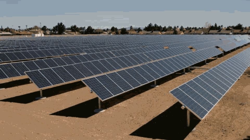
Economic Feasibility of Solar Photovoltaic Irrigation Systems
The Great Basin is primarily located in Nevada, western Utah, and small sections of southern Oregon and Idaho. The Great Basin is noted for its arid conditions and high percentage of publically owned land. The potential for solar energy generation in the
Energy Conservation with Irrigation Water Management
Irrigators in Utah experienced rapidly increasing energy costs from the mid 1970s to the late 1980s. These costs remain relatively high. Those who are pumping from deep wells are particularly interested in ways to cut back on energy use without doing away
Guide to Irrigation Sprinkler Packages for Pivots and Laterals
Guide to Irrigation Sprinkler Packages for Pivots and Laterals
How Good is Your Water Measurement?
Accurate water measurement is essential to maintaining equity of water delivery within an irrigation company or water districts. Good management of our scarce water resource is dependent upon quantifying supplies and uses with accurate measurement techniq
Irrigation Canal Lining?
Irrigation canals placed in native soil or lined with earth can have seepage water losses varying from 20 percent to more than 50 percent. Well designed, new compacted earth lined canals can have reduced seepage losses similar to concrete lined channels.
Irrigation Water Loss and Recovery in Utah
When deciding which irrigation systems to adopt, permit, or promote, it is important to consider how their efficiency and losses affect the water balance of Utah’s watersheds and drainage basins. Irrigators have no control over precipitation and only limi
Irrigation Water Quality Sampling Guide
The suitability of a water source for irrigation depends on the water quality, and some sources may be altogether unsuitable for practical use.
Managing Saline and Sodic Soils and Irrigation Water
Salt is important in plant and soil management. Excessive salt concentrations in soil can cause water to be less available to plants because of the osmotic forces of salt in the soil water. Excessive concentrations of some salt ions can also be toxic to p
Managing Soil pH for Crop Production in Calcareous-Alkaline Soil
In semiarid soils of the Western U.S., altering soil pH is not easily accomplished nor straightforward. Recall that pH is a measure of the acidity or alkalinity of a substance. More specifically, Utah’s soil pH range can be 1,000 times more acidic or alka
Mobile Drip Irrigation for Pivots and Laterals
New technologies like MDI have the potential to improve irrigation efficiency thereby increasing water available to the crop and conserving water by reducing loss. If you are considering MDI on your farm, it will be important to carefully review its poten
Precision Irrigation Guide for Center Pivots
Precision irrigation is a process involving technology and specialized equipment to improve the efficiency and effectiveness of agriculture irrigation management. This management process is beneficial in allocating water based on spatial variability throu
Soil Sampling Guide for Crops
Why conduct soil sampling for crops? The answer is simple and intuitive for most involved in agriculture. Regular soil sampling, testing, and associated guidance on fertilization and soil amendments help develop and maintain more productive and healthy
Strategies for Deficit Irrigation of Forage Crops
Deficit irrigation strategies with varying effectiveness can be employed in many cases to maximize production and profit. These strategies can include modifying irrigation schedules, concentrating irrigation to critical crop growth stages, reducing rates,
Ten Considerations for Solar-Powered Irrigation in Utah
Generating power from solar energy used to be one of the most expensive options in Utah. This scenario is changing. According to the American Council on Renewable Energy (ACORE, 2021), the cost of solar power production went down by 90% between 2009 and 2
Understanding Irrigation Water Optimization
It is important to consider the possible hydrologic impacts of irrigation optimization efforts to avoid implementing practices that have little appreciable effect relative to the desired outcome. Examples of desired outcomes include increasing supply reli

Utah Surface Irrigation Water Optimization Opportunities and Barriers
This peer-reviewed fact sheet from Utah State University Extension summarizes a statewide survey of surface irrigators, highlighting current practices, barriers, and opportunities for water optimization in Utah agriculture. It emphasizes the importance of
Variable Frequency Drives for Irrigation Pumps
A VFD can make sense in a variety of irrigation applications. Here are 6 of the major applications where one might consider a VFD (also see Henry and Stringham, 2013 and USDA-NRCS, 2010):
Water Rights in Utah
If you are connected to a municipal system, your water is probably categorized as “culinary or municipal water” and is used for everything from drinking and bathing to washing the car to watering tomatoes. However the Utah Division of Water Rights takes a
25 Rules of Thumb for Field Crops
University Extension services are widely known for scientific information on best practices for field crop production. Many Extension experts commonly offer the same tips or "rules of thumb" to growers. This article is certainly not a comprehensive list o
Irrigation Advance Sensors Are Having Large Impacts in Surface Irrigation
There are many good things about surface irrigation, but the labor requirements and large water withdrawals can diminish its feasibility in situations with limited access to labor or water. In this fact sheet, we will describe two of these systems current