Value Landscape Engineering
Identifying costs, water use, labor, and impacts to support landscape choice
David E. Rosenberg, Assistant Professor, Department of Civil and Environmental Engineering and Utah Water Research Laboratory;
Kelly Kopp, Professor/Extension Water Conservation, Turfgrass Specialist;
Heidi A. Kratsch, Assistant Professor, University of Nevada Cooperative Extension, Reno, Nevada;
Larry Rupp, Extension Landscape Horticulture Specialist;
Paul Johnson, Department Head, Professor of Turfgrass Management/Genetics;
Roger Kjelgren, Professor, Department of Plants, Soils and Climate
Abstract
We present a spreadsheet model that identifies the costs, water, labor, fertilizer, pesticides, fuel, energy, carbon emissions, and particulates required of and generated by a user-specified residential or commercial landscape over its economic life. This life includes site preparation, materials purchase, installation, annual maintenance, and replacing landscape features that wear out or die. Users provide a variety of site-descriptive information, and the model queries an extensive database of landscape data to calculate costs, required inputs, and impacts. We verified model results against observations of water, labor, fertilizer, and fuel use over eight years at three landscapes in the Salt Lake City (SLC), Utah metropolitan region. We use the model to show tradeoffs in costs and required inputs for a predominately cool-season turfgrass landscape typical for SLC and other high desert, intermountain western U.S. cities and potential modifications to that typical landscape. Results highlight strategies water conservation programs can use to encourage property owners to install and adopt water-conserving landscape features and practices. Residential and commercial landscapers, landscape architects, contractors, and property owners can also model current and proposed landscapes and use results to identify a low-cost, low-input landscape that achieves their client’s or their own goals and values.
Key Terms: outdoor water use; required labor, fertilizer use, pesticide use, fuel use, energy use, CO2 emissions, particulate emissions, landscape choice, spreadsheet model, value engineering.
Introduction
Outdoor water use comprises a large portion of deliveries for many western municipal water utilities, and utilities are stepping up efforts to improve urban landscape irrigation efficiency. Many utility conservation programs have targeted behaviors associated with irrigation. Examples include ordinances to limit when people can water, outreach programs to help educate customers about plant water needs, landscape irrigation evaluations to help improve the application efficiency of irrigation systems, rebates to help offset costs to connect irrigation controllers to weather sensors (Mayer et al. 2009), and water-budget-based rate structures (Mayer et al. 2008). Except for the turfgrass buyback program sponsored by the Southern Nevada Water Authority, few conservation programs have targeted landscape composition: changing what residential- and commercial-property owners plant and where.
Efforts to change landscape composition have been limited for several possible reasons. First, property owners often overwater (Endter-Wada et al. 2008), regardless of landscape composition. Changing irrigation behaviors to meet rather than exceed plant water needs can yield significant water savings. Second, utilities assume that property owners have already decided what kind of landscaping they want and owners want to keep what they currently have. Third, urban landscapes are complex systems. Plant composition, site-specific conditions, and maintenance activities interact in many ways so that it is difficult to determine the effect on water use of changing one or more landscape system components. And fourth, little information is available to property owners about the impacts of changing one or more landscape components on their overall water and energy consumption. Costs, required labor, fertilizer, fuel, pesticide and energy use, carbon dioxide (CO2) and particulate emissions, aesthetics, and other attributes may also influence property-owner landscape choices. Further, existing information is dispersed among scientific and university Cooperative Extension sources, vendors, and landscape professionals, and is not organized or synthesized to support decision-making by property owners.
To address some of these limitations and support property owner landscape decisions, we have developed a spreadsheet model that identifies the costs, required labor, water, fertilizers, pesticides, energy, fuel, carbon emissions, and particulates required for, or generated over, the life of a user-specified landscape. This life includes all onsite landscaping activities such as preparing the site, purchasing and installing materials, annual maintenance and operations, and replacing features and components that wear out or die. Modeled landscape features and components include drought tolerant and intolerant trees, shrubs, ground cover, turfgrass, perennials, annuals, and vegetable gardens. In addition, hardscaping, decks, irrigation systems, fencing, and rock walls are also considered. The model quantifies costs, inputs, and impacts in easy-to-understand units such as dollars, gallons, pounds, hours, kilowatt-hours, pounds of CO2 or particulate matter, square feet, cubic feet, and cubic yards. Landscapers, landscape architects, contractors, and owners of residential and commercial properties can use the model to identity costs, required inputs, and impacts for a current landscape, landscape plan, or modifications to them. This information can help property owners (who are willing to invest the time and effort) determine a preferred landscape.
The spreadsheet model fully implements the concept of value landscape engineering (VLE). The VLE concept was introduced over a decade ago (Rupp et al. 1997a; Rupp et al. 1997b) and sought to consider all activities associated with a particular landscape over its life. The goal was to maximize value and reduce required inputs. Until now, VLE faced major challenges to adoption: (i) it required onerous calculations by hand, and (ii) limited information was available on several inputs and impacts. The VLE concept is analogous to land-use system modeling (Rosenberg and Marcotte 2005; Vosti et al. 2000) and similar to life cycle assessment (LCA)(USEPA 2006). Like LCA, VLE considers all onsite activities over the life of the landscape but, unlike LCA, ignores costs, inputs, and impacts to produce materials, transport them to the site, and dispose of waste materials offsite. We restricted the VLE model scope to on-site activities, associated costs, inputs, and impacts, to best support property owner choices regarding landscaping.
The spreadsheet model for download, user manual, sample application, and a web version are available online at http://vle.cuwcd.com. Model default settings, data, and verification have focused on residential and commercial landscapes in the Salt Lake City (SLC), Utah metropolitan area. But the model is general and readily applied to other cities in the high desert, intermountain, western U.S. region. Still, we recommend further testing and verifying the model prior to using it in new cities or regions. Herein, we (i) describe the VLE model organization, data, and calculations, (ii) verify model results for three SLC metropolitan landscapes against observations over eight years of water, labor, fertilizer, and fuel use, and (iii) use the model to show value tradeoffs for several water conserving landscapes and landscape practices common in SLC and the region. Section (iv) concludes by recommending strategies for conservation programs to encourage water conserving landscapes.
Model Organization
The VLE model determines costs, required inputs, and impacts of all landscape features over each landscape life stage (Table 1). Features include major and sub-categories of planted and hardscaped areas (Table 2), irrigation and lighting systems, fencing, and rock/retaining walls. These features and sub-categories were chosen to (i) represent a wide range of common landscaping attributes, (ii) provide a level of disaggregation that could identify tradeoffs in required inputs or impacts among landscape features, (iii) be understood by model users, (iv) use available data, and (v) further educate users about landscape features that can conserve water.
The spreadsheet program first prompts the user to enter initial assumptions about their landscape such as the number of years for the analysis (economic life of the landscape), interest rate to discount future costs, prices for all inputs, percentage of labor that will be hired out, current summer and winter energy usage, and length of the growing season. Second, users enter the total landscaped area (in square feet) and the coverage of each landscape feature (as a percentage of the total landscaped area). The user must also enter unit prices and the lifespan (number of years until replacement) for each landscape feature, or leave values at default settings. Users select the irrigation systems and maintenance equipment and specify the desired maintenance level (conventional or intense). This maintenance level refers to the frequency of several maintenance activities and the amounts of inputs used. The “conventional” level is appropriate for most do-it-yourself homeowners and assumes turf is mowed once per week, planting beds weeded once per month, turf edged twice per year, and leaves raked and hedges trimmed once per year. The “intense” level represents maintenance typically practiced by landscape and lawn care companies. This level doubles the frequency of turf-mowing, edging, leaf-raking, and hedge trimming; quadruples weeding; aerates turf and rototills vegetable gardens annually; and fertilizes and waters turf and applies pesticides and herbicides at 1.2 to 1.3 times the “conventional” rates.
Subsequently, the program queries a database we assembled of required water, labor, fertilizer, pesticide, and other inputs per unit area for each landscape component and then calculates costs, required inputs, and outputs on an annual basis and over the economic life of the landscape. A User’s Guide details model use and features (Rosenberg et al. 2009). Here, we discuss the data and calculations that estimate landscape costs, required inputs, and impacts.
Costs
Costs are expressed in today’s dollars ($US 2009) and include one-time capital costs in the first year to prepare the site and purchase and install materials, plus recurring costs in the first and subsequent years to operate and maintain the landscape over its economic life. Additionally, replacement costs (materials purchased and re-installed) are tabulated for each landscape component at the appropriate point in the future based on the lifespan the user specifies for each landscape component.
Costs are calculated by multiplying the unit price for each landscape feature or input ($/unit) by the number of required units. The user specifies the number of required units for landscape features as part of defining the landscape coverage and configuration. The program calculates other inputs, such as water, labor, energy, fuel, etc. (see later sections). We compiled default prices and life spans for inputs and landscape features after consulting a variety of landscaping firms, nurseries, sod farms, irrigation firms, building supply companies, arborists, and water and electrical utilities in the greater SLC metropolitan area. We also consulted product listings on Lowes, Home Depot, Sears, and John Deere websites and cost and price information in R.S. Means Site Work and Landscape Cost Data (Balboni 2001).
The standard discounting formula is used to reflect the time-value of money and convert all future costs for operations, maintenance, replacements, and removals into present value costs. Discounting allows users to compare future and immediate costs (such as for site preparation and installation) as well as landscapes that incur costs at different points in time. The discounting formula is:
(Eq. 1)
cp = cft(1+i) -t
Where cp = the cost of the item at present ($ present), cft = the cost of the item in future year t ($ future), i is the interest rate (fraction), and t is the number of years in the future when the cost will occur. The user enters the interest rate i for the analysis as part of the initial assumptions and to reflect his/her financial circumstances. The number of years in the future t is either (i) all integers 1 through the user-specified economic life of the landscape (for annual operations and maintenance activities and inputs associated with those activities), or (ii) the user-entered life of a landscape component and all multiples of that life that are less than the economic life of the landscape. Capital costs and discounted future operating and replacement costs are distilled into a bottom-line, present value of all costs.
Water Use
Landscape irrigation water use is quantified in gallons and estimated from annual plant water requirement factors for a reference growing season in the intermountain western U.S. (Appendix A) (Cerny et al. 2002; Fortier and Belt 1998; Kneebone et al. 1992; Kratsch et al. In press; Moller and Gillies 2008). We estimated water requirements for non-turfgrass plants by multiplying the (i) average crown diameter of a single plant or of a homogeneous planting, (ii) average reference evapotranspiration (ETo) for north-central Utah during the growing season, and a (iii) plant factor. The plant factor is a dimensionless fraction of ETo and derived from studies that show many conventional landscape species maintain their health and appearance when irrigated within a range of 20 to 80% of ETo (Pittenger et al. 1990; Pittenger et al. 2001; Shaw and Pittenger 2004; Staats and Klett 1995). Turfgrass water requirements were also calculated from historic ETo rates for the region, but used plant factors of 80 and 60% for cool and warm-season grasses, respectively. These plant factors were also adjusted for the selected maintenance level.
We prorate plant water requirement factors for the reference growing season length (120 days for annuals and vegetables; 180 days for other plants) by the growing season length specified by the user, then divide by the irrigation efficiency of the irrigation system component the user selects for each plant zone within the landscape. The model uses average irrigation efficiency rates of 85 and 78% for drip systems and above-ground sprinklers (Liljegren, pers. comm., 2009). If choosing an in-ground irrigation system, the user must also select an efficiency rate between 40 and 80%.
Plant water requirement factors for year 3 and beyond assume that trees get sufficient water from the turfgrass or shrub area surrounding the tree. For most other planting types, we differentiate annual water needs in year 1 from year 2 and beyond. These establishment and subsequent-year water requirement factors repeat in time according to the lifespan (years) a user specifies for the landscape feature. Total landscape irrigation water use is the sum of annual irrigation requirements for all plant areas over the economic life of the landscape.
Labor
Labor is quantified in hours and divided among the different landscape life stages. Labor for site preparation (hours) includes grading, ripping, excavation, and topsoil addition. The user specifies the task size (required units in square feet or cubic yards). Then, the spreadsheet program multiplies each task size by task rate data (hours/unit to operate the equipment such as a front end loader, skid steer, or grader) to determine the hours of operation.
Installation includes labor (hours) to place planting materials or hardscapes, set up irrigation and lighting systems, and build walls and fences, and is also calculated by multiplying task sizes by task rates (hours/unit). Task sizes derive from user-specified landscape feature coverage (such as square feet of turf area) or the required units (such as number of trees). Task rates for some activities such as deep trenching to lay irrigation pipe reflect use of equipment, while other tasks such as planting are manual.
Maintenance labor (hours/year) is calculated by multiplying task rates (hrs/unit), the number of specified units, and the frequency (times/week, month, or year) the task is performed. Maintenance includes labor to prune trees and shrubs, remove dead perennials and annuals, weed, apply pesticides and herbicides, and mow, edge, blow, and fertilize turf. Should a user select above-ground hoses and sprinklers to irrigate one or more plant zones, there is additional labor required to move the hoses and sprinklers. The user’s selection of the desired maintenance level determines the frequency maintenance tasks are performed.
Finally, labor to remove and reinstall landscape features (hours/replacement) is calculated by multiplying required units and task rates. For example, when fast-growing trees die, they need to be taken down and the stump removed. A new tree is then planted. Similarly for shrubs, perennials, ground covers, and other landscape structures and systems. Task rates for reinstallation are the same as for the initial installation.
We use labor task rates in existing publications (Thompson and Sorvig 2008) or provided by professional landscapers, arborists, and grounds crews who have recorded the time to perform tasks using different equipment in a variety of conditions over many years (Ashby, pers. comm., 2009; Aston, pers. comm., 2009; Malmstrom, pers. comm., 2009; Peterman, pers. comm., 2009). This detail also allowed us to embed economies-of-scale in the model—using bigger equipment to complete larger tasks at a faster unit task rate. Where observation data was not available, we estimated task rates by dividing cost estimates (Balboni 2001; PGMS) by a hired labor rate of $40/hour.
Total labor is sum of labor for (i) site preparation, (ii) installation, (iii) annual maintenance multiplied by the economic life of the landscape, and (iv) removal and reinstallation multiplied by the number of reinstallations. The number of reinstallations for a landscape feature is one less than the economic life of the landscape divided by the lifespan of the feature rounded down to the next integer. For example, over an 8-year economic life and analysis period, a landscape feature such as mulch with a life span of 3 years would need to be replaced twice (in the 4th and 7th years; round-down [(8 – 1)/3] = 2).
Fuel
Fuel use is quantified in gallons and calculated by multiplying for each labor task that uses fossil-fuel powered equipment, the (i) hours to complete the task (see Labor above), (ii) engine horsepower, and (iii) a conversion factor that specifies fuel consumption per horsepower-hour (Thompson and Sorvig 2008). The model differentiates equipment and fuel consumption for diesel, gasoline, and gasoline-oil engines using conversion factors of, respectively, 0.06, 0.08, and 0.09 gallons/horsepower-hour for each fuel (Thompson and Sorvig 2008).
Tasks requiring equipment and thus fuel include all site preparation tasks, trenching for in ground irrigation (if the trench is deeper than 12”), building rock / retaining walls, and removing fast-growing trees. The following operations and maintenance tasks also use fuel: trimming hedges; rototilling perennial, annual, and vegetable gardens; and aerating, mowing (if a gasoline powered mower is selected), blowing (if a blower is selected), and edging turfgrass areas. Equipment economies-of-scale also affect fuel use and are included by using the engine horsepower specific to the labor task rate used to calculate labor.
Non-Fuel Energy Use
Net energy use is quantified in kilowatt-hours (kW-hr) and is estimated as the energy used by electrical equipment to maintain the landscape minus the energy saved from reduced heating in winter and cooling in summer. When electrical maintenance equipment (such as an electric lawnmower) is selected, the model calculates annual energy use (kW-hr/year) by converting the equipment engine’s horsepower rating to kilowatts then multiplying by the hours per year equipment is used (see Labor, above). We assume energy savings accrue when certain types and numbers of trees are planted near a house or building. The model calculates savings as a percentage of existing metered energy use (also entered by the user). Energy savings accrue when a user indicates they will plant:
- At least three deciduous trees within 3 feet of the building on the south or west sides, or
- At least 6 coniferous trees on the north or east side of the house or building.
Deciduous trees planted on the south or west sides of a building can shade the building in summer, reducing the energy expended to cool it, and decrease total building summer energy use by 10% (Akbari et al. 2001; Dimoudi and Nikolopoulou 2003). This reduction does not consider the cooling effects of turf located near a building. In winter, deciduous trees lose their leaves, allowing daytime sunlight to enter a building and warm it and reducing the energy expended to heat the building, and decrease total winter energy use by 10% (Akbari et al. 2001; Dimoudi and Nikolopoulou 2003). Coniferous trees planted on the north or east side of a building can block winter wind, reduce the energy expended to heat the building, and decrease winter energy use by 20% (Akbari et al. 2001).
Fertilizer
Fertilizer use is quantified as pounds of nitrogen and estimated from annual plant nitrogen requirement factors (Appendix A) (Fitzpatrick and Guillard. 2004; Frank et al. 2004; Hensley 2005; Johnson et al. 2003; Turner and Hummel 1992). The model assumes trees have lower nitrogen requirements than the other plant features and that trees obtain sufficient nitrogen from the fertilizer applied to the plants surrounding the tree. The model requires turf be fertilized, but the user can choose to not fertilize shrubs, perennials, annuals, ground cover and/or vegetable garden and assume that the breakdown of organic mulches applied to these areas provides sufficient nitrogen. We multiply the annual nitrogen requirement factor by the number of shrubs or square footage for other planting areas and by the economic life of the landscape to obtain the total required nitrogen.
Pesticide Use
Pesticide use is quantified in pounds of active ingredient and differentiated by herbicides, insecticides, and fungicides. Annual application rates are based on recommended treatment schedules for common landscape pests in Utah (Appendix A) (Surflan, 2009, http://www.afpmb.org/pubs/standardlists/labels/6840-01-318-7417_label.pdf; Lowe's; Home Depot; UC Davis, Integrated Pest Management Program, http://www.ipm.ucdavis.edu; Glyphosate, 2009, http://www.umt.edu/sentinel/roundup_label.pdf; Iowa State University Weed Extension, 2009, http://www.weeds.iastate.edu/mgmt/2001/glyphosateformulations03.htm,; http://utahpest.usu.edu; Sevin, 2009, http://www.gardening123.com/ProductInfo/sevin/PestList.asp?TM=2&PestCat=1; Aston, pers. comm., 2009). Total pesticide use is calculated by multiplying recommended annual application rates by the planting areas and by the economic life of the landscape.
Carbon Footprint
The carbon footprint is quantified in pounds of net carbon dioxide emissions. Emissions are from all labor activities that use fuel-powered equipment (see Fuel above). Diesel fuel generates about 22.2 pounds of carbon dioxide per gallon burned while gasoline and gasoline-oil fuels generate only 19.4 lbs of carbon dioxide per gallon burned (Coe 2005). Carbon emissions are calculated by multiplying the emissions rates by fuel used (see Fuel above).
Net carbon emissions are the carbon emitted by landscape equipment burning fuel minus the carbon sequestered by landscape plants. Here, we use annual sequestration rates of 50 pounds per tree, 8 pounds per shrub, and 0.07 pounds per square foot of turf, groundcover, perennials, vegetable garden, and annuals (Huh et al. 2008; McPherson and Simpson 1999; Qian and Follett 2002; USFS 2009). Of the plant materials considered, trees take up and store the most carbon in wood. Turf—because of longevity, high rooting density, and organic matter deposition—may sequester more carbon than herbaceous perennials, annuals, ground covers, or vegetables, but more detailed carbon sequestration data for these plant types is not currently available. Calculated hydrocarbon output is negative when landscape plants sequester more carbon than is emitted to install and maintain them.
Particulates-Dust
Dust or particulate emissions are quantified in pounds of particulate matter greater than 10 microns and calculated directly from equipment fuel use. Particulate emission from gasoline and diesel fuel is calculated by multiplying the gallons of diesel and gasoline (see Fuel above) by 0.006 pounds PM 10 per gallon of fuel (NPI 1999). The conversion factor for gasoline-oil fuel is 0.054 pounds PM 10/gallon, and is 10 times that for diesel and gasoline because oil does not completely combust (NPI 1999). Gasoline-oil engines include string trimmers, lawn edgers, and blowers for turf; and reciprocating trimmers and chain saws for shrubs and trees.
Model Verification
We verified VLE model results against observations of water, labor, fertilizer, and fuel use at three landscapes located in the “Neighborhood” section of the Jordan Valley Water Conservancy District (JVWCD) Conservation Garden Park in SLC. The Neighborhood section emulates a residential street having different themed yards or landscapes. We chose the Traditional, Perennial, and Woodland Landscapes for verification since these landscapes have varied plant types, irrigation systems, and maintenance requirements.
Each Neighborhood landscape is metered separately to help track and compare water use among landscapes. We gathered planting area, planting coverage, and layout information from JVWCD staff and entered values into the VLE model. We also collected staff observations of water, labor, fertilizer, and fuel inputs for each landscape beginning in 2001, when the landscapes were established, to 2008. JVWCD staff only had observations of fuel and labor use for the entire Neighborhood area and estimated uses for each landscape. JVWCD staff does not record pesticide or energy use or particulate or hydrocarbon outputs, so these model results were not verified for the landscapes.
To model these landscapes, we generally used VLE model default settings except for the Economic Life of the Landscape. We changed this value to eight years to match the number of years for which observational data were available. We selected an “intense” maintenance level as JVWCD has staff to maintain the landscapes, but we also revised some maintenance levels to more accurately reflect the times and frequencies JVWCD staff perform and do not perform several activities: mowing turfgrass once per week, edging and blowing all areas once per week with a string trimmer and blower, fertilizing only turf areas, weeding all areas (including turf) by hand, and not rototilling or applying pesticides. Table 3 shows the landscaped areas and planting coverage in the three landscapes. Below, we describe each landscape and compare VLE model results to JVWCD observations.
Landscape descriptions
Traditional Landscape
The Traditional Landscape in the Conservation Garden Park resembles a traditional intermountain west landscape choice and has a large cool-season turfgrass area, some drought tolerant shrub beds, drought-tolerant and drought-intolerant perennial beds, paved walkways, drought-tolerant ground cover, and several trees. An in-ground sprinkler system operating at peak efficiency irrigates the entire landscape.
Perennial Landscape
The Perennial Landscape uses perennial plants, some shrubs, ground cover, and paved areas. It has a much smaller area of cool-season turfgrass than the Traditional Landscape. In-ground sprinklers irrigate the turf area, while a drip system irrigates the remaining planting areas.
Woodland landscape
The Woodland Landscape has only trees and drought-tolerant shrubs and perennials. It is irrigated entirely by a drip system, has no turfgrass, and is an example of a dry shade garden.
Comparing VLE model results to JVWCD observations
Water use
For the eight-year comparison period, observed and modeled water uses for each landscape are similar (Table 4). We used the root mean squared error (RMSE) to quantify model error which was 13,800 gallons/year. Mathematically, RMSE is the average squared differences between modeled (Ml,t) and observed (Ol,t) annual water use in the three landscapes l over the seven post establishment years t included in the error estimate (Eq. 2).
(Eq. 2)
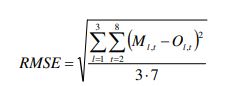
The RMSE of 13,800 gallons/year is small compared to observed annual water uses for the three landscapes which averaged 73,000, 49,000, and 20,000 gallons/year for the Traditional, Perennial, and Woodland landscapes. A residual analysis (Ml,t - Ol,t) suggests annual differences are independent, normally distributed, and have similar variance through time. However, the model consistently underestimates annual water use by the Perennial Landscape. This landscape has much larger areas of perennials than the other landscapes, and the discrepancy may occur because either (i) the VLE model uses annual post-establishment water requirements for perennials that are too low, or (ii) JVWCD garden staff overwatered this landscape relative to its water requirements. Otherwise, model estimates and observations of water use at the three landscapes are similar and verify against one another.
Labor
Observed and modeled estimates of annual labor for the three landscapes are within 30% of each other (Table 5). Modeled estimates also verify against observations that show the Perennial Landscape requires the most labor and the Woodland Landscape the least, even though the VLE model still over- and under-estimates labor amounts for these two landscapes. These results may occur because JVWCD staff weed (i) perennial beds by hand at a slower rate than the task time rate used by the VLE model, or (ii) shrub beds at a faster rate than the task time rate used by the model. VLE model estimates and observations for labor differ significantly when using default timings and frequencies to rototill, apply pesticides, fertilize non-turf areas, mow, blow, weed, and edge turf, and weed and blow all other areas (results not shown, see Rosenberg et al. (2009)). These findings suggest model results are sensitive to the frequencies (over a growing season) that labor activities are performed.
Fertilizer use
Observed and revised modeled nitrogen estimates are the same (Table 5). Here, JVWCD staff apply 4 pounds of nitrogen fertilizer per 1000 ft2 of turf which is the same value used by the VLE model for the “conventional” maintenance level. If the “intense” maintenance level is used, which assumes a turf application rate of 6 pounds nitrogen fertilizer per 1000 ft2, the VLE model overestimates required nitrogen by about 50% (results not shown, see Rosenberg et al. (2009)). This finding again emphasizes that VLE model results are sensitive to the maintenance level—both the frequency that labor activities are performed and intensity with which inputs are used.
Fuel use
Model estimates for gasoline and gasoline-oil fuel use by the Traditional and Woodland Landscapes are generally within 30% of each other (Table 5). While observed and estimated total fuel uses are close, the VLE model estimates gasoline fuel use in the Perennial Landscape significantly below the observed value. This difference may be because JVWCD staff incorrectly figured gasoline use at 1.5 gallons/year for the Perennial Landscape. The lawnmower is the only gasoline-powered equipment JVWCD staff use in any of the landscapes. The Perennial Landscape has 1/9 the turfgrass area of the Traditional Landscape, yet the observed gasoline fuel use is only 1/3 the Traditional Landscape (1/9th the gasoline use of the Traditional Landscape would be approximately 0.5 gallons/year and nearly identical to the modeled estimate). Additional differences could occur because the model uses an incorrect horsepower engine rating for the gasoline-oil powered blower and string trimmer, or because JVWCD staff blow and string trim at rates slightly faster than the task rates used by the model.
Model Results
We now use the VLE model to estimate costs, required inputs, and likely impacts and show tradeoffs among them for several water-conserving landscape options. This use reflects how a user typically interacts with the spreadsheet program: first enter an existing landscape or landscape plan, then, evaluate modifications to it.
Here, we set the “existing” (base case) landscape to be a predominately cool-season turfgrass such as Kentucky bluegrass (80% of the landscaped area) with smaller hardscape (10%), drought-tolerant shrub (5%) and perennial (5%) areas. This composition represents many turf dominated residential landscapes in SLC and the high desert, intermountain region. We use a total landscaped area of 10,000 sq. ft., 15 fast- and slow-growing trees and conifers scattered throughout, and an in-ground sprinkler system operated at 60% efficiency. We also assume there are no site preparation activities, a 25-year life for the landscape, 3% interest rate, conventional maintenance level, fertilization of turfgrass areas only, and that the owner provides all labor. All other model parameters are set at their default values.
The VLE model estimates total present value costs over the 25-year life of the landscape at $46,000. The landscape will also require 6.3 million gallons of water, 6,300 hours of labor, 500 gallons of fuel, and 800 pounds of nitrogen as fertilizer.
Warm-season turfgrass
One water-conserving option is to plant a warm-season turfgrass such as buffalograss [Bouteloua dactyloides (Nutt.) J. T. Columbus] or blue grama [Bouteloua gracilis (B.B.K.) Lag. Ex Steud.] instead of the cool-season turfgrass used in the “existing” landscape. The VLE model results show that a warm-season turfgrass landscape costs less over a 25-year period, has lower annual costs, and requires less water, nitrogen, and labor than a cool-season turf landscape (Table 6). Although warm-season turfgrass costs more to purchase ($0.15/sq. ft. to seed compared to $0.06/sq. ft. for cool-season turfgrass, (Biograss Sod Farms, pers. comm., 2009), this extra initial cost is offset by reduced payments for, and use of, water. In fact, either the purchase price would need to rise to $0.30/sq. ft. or the price of water would have to drop to $0.50/1000 gallons to make cool-season turfgrass financially preferable (Figure 1). For numerous water and warm season turf purchase prices, substituting warm-season turf can yield thousands of dollars in financial savings over the 25-year life of the landscape. Savings increase by $1,600 per $1 increase in the price for 1,000 gallons of water. These VLE model results show that warm-season turfgrass can cost less over the life of a landscape plus save water, labor, and fertilizer compared to an identically-sized cool-season turfgrass landscape.
Reduce turfgrass area
A second water-conserving landscape option is to reduce turfgrass area. Here we examine converting turfgrass to either (i) equal areas of planted drought-tolerant shrubs and perennials, or (ii) hardscape.
As turfgrass coverage is reduced from 80% (in the “existing” landscape) to 0% (no turfgrass), water use falls but total costs nearly double (when replacing all turfgrass with hardscape) or triple (when replacing with shrubs and perennials) over the life of the landscapes (Figure 2). Note, the existing landscape already has hardscape, shrubs, and perennials (10%, 5%, and 5% coverage), so reducing turf area also increases shrub/perennial or hardscape coverage from 10% to 90%. Total costs rise sharply because hardscaping, shrubs, and perennials are more expensive to purchase per square foot and because perennials, mulch, and some shrubs must be replaced more frequently than turf. But choosing the right mix of plants to substitute for turf is also important. For example, substituting long-lived drought-tolerant shrubs for all turf only increases total costs by a factor of 2 not by 3. Figure 2 also highlights other important tradeoffs among inputs. First, annual costs fall as shrubs, perennials, and hardscape require less fuel and other inputs than turf. Second, shrub and perennial landscapes require less labor to maintain than turf, but require significantly more labor over the landscape life to install, replace, and reinstall plant materials. And third, there is slight decrease in net CO2 sequestered when substituting hardscape for turf and a large increase when transitioning to shrubs and perennials. These results show that conventionally maintained turf is a net carbon sink; but this finding is sensitive to the maintenance level and carbon sequestration rate assumed (Townsend-Small and Czimczik 2010).
More intense management
Property owners may also want to know the additional costs, labor, and other inputs associated with the improved look of a more intensely managed landscape. Comparing VLE model results for (i) the conventional maintenance level in the “existing” landscape to a (ii) more intense level shows that required labor, water, and other inputs significantly increase (Table 7). Hydrocarbon output also increases as net carbon sequestered by the landscape decreases. Total costs over the 25-year life of the landscape only increase by about $3,600. However, this amount assumes the property owner performs all the additional labor. If the additional 103 hours per year of labor for more intense management over 25 years is hired out at $40/hour, then total present value costs increase by $72,000.
Discussion
VLE model results highlight several findings regarding landscape practices and composition to encourage water conservation which we elaborate upon here. First, landscapes require significant money, time, water, fertilizers, and other inputs over the long (often exceeding 25-year) period that people may own a residential or commercial property. Second, replacing cool-season turfgrass with warm-season turfgrass can substantially reduce total and annual costs, water, labor, and fertilizer use over a wide range of water and turf seed prices. Water conservation programs should emphasize these multiple benefits of warm-season turf. However, programs must also caution that in northern climates, warm-season turfgrass has a shorter growing season, is dormant during spring and fall, and may not be aesthetically pleasing or suitable for intense recreational use then. Third, replacing cool-season turf with drought-tolerant shrubs or perennials or hardscaping can significantly decrease water use and net CO2 emissions. This substitution will also change total costs and required labor with changes dependent on both the plant material substituted and planting density. For example, lowering the planting density and increasing mulched areas can reduce installation and subsequent maintenance cost, allow more rooting volume per plant, increase soil water availability, reduce irrigation water use, and enhance drought tolerance. Thus, water conservation programs may want to emphasize replacing only small areas of turfgrass and replacing turf with long-living drought-tolerant shrubs at low planting densities. Fourth and finally, VLE results show that intensively managing a landscape can significantly increase all costs, required inputs, and impacts. But property owners can realize large savings if they follow recommended maintenance practices.
Limitations
The results and discussion are based on VLE analysis over 25 years for a predominately cool season turf landscape in the SLC area and select modifications to it. Changes in the economic life, landscaped area, purchase prices and lifespans of landscape components, frequency of maintenance activities, or other default settings may affect the magnitude of results but not the overall trends. Focusing on the relative changes in costs, inputs, and impacts among landscape
options will reduce input data specification errors and systematic model biases. Further,
- Model data, default settings, and testing to date have been exclusively for SLC, Utah metropolitan area landscapes. The model is readily applied in other cities in the high desert, intermountain region, but we recommend further testing and verifying the model in new locations prior to use there.
- Whenever possible, model users should substitute site-specific and appropriate values for default settings.
- Some impacts of on-site activities, like water quality, runoff, and fate and transport of groundwater and groundwater contaminants, are excluded due to data and computational limitations.
- The model is most readily used by residential and commercial landscapers, landscape architects, contractors, and managers familiar with landscape terms and activities. Home and business owners can use the model, but may need to invest more time and effort.
Conclusions
We have developed a value landscape engineering spreadsheet model that identifies costs, required inputs, and impacts over the specified economic life of a residential or commercial landscape. This life includes site preparation, purchasing and installing materials, annual maintenance, and replacing landscape features that wear out or die. Users provide a variety of site-descriptive information including the total landscaped area, planting coverage, maintenance level, and prices and lifespans for each landscape component. Then, the model queries an extensive database of landscape data for Utah and calculates the costs, labor, water, fertilizers, pesticides, energy, fuel, carbon emissions, and particulates required for or generated over the life of the user-specified landscape.
Model results verify against observations of water, labor, fertilizer, and fuel use over eight years at three landscapes in the Jordan Valley Water Conservancy District Conservation Garden Park in the SLC metropolitan area, Utah. Verification also shows that model results are sensitive to the frequencies maintenance activities are performed. To date, model data and testing have focused in the SLC area; while readily applied in other locations, we recommend further testing and verifying the model in new locations prior to use there.
We demonstrate model use for a predominately cool-season turfgrass landscape typical for SLC and other high desert, intermountain western U.S. cities plus potential modifications to the typical landscape to conserve water. Model results suggest:
- Substituting warm-season turfgrass can synergistically save water, money, time, and fertilizer.
- Replacing turfgrass with shrubs and perennials is expensive. Water conservation programs should recommend replacing only small areas of existing turf with drought tolerant shrubs and installing shrubs at low planting densities.
- Property owners can realize substantial savings if they adopt recommended landscape maintenance practices.
Landscapers, landscape architects, contractors, and property owners can also use the model to identify costs, required inputs, and impacts for a current landscape, landscape plan, or modifications to them. This information can help them or their clients choose a landscape that achieves the VLE goal of maximizing value and reducing required costs and other inputs.
Appendix A. VLE Model Data for Water, Fertilizer, and Pesticide Inputs
Annual water requirements used by the VLE model for each planting type sub category are listed in Table A1. Table A2 shows the fertilizer and pesticide requirements for each planting type sub category.
Table A1. Annual water requirements for VLE model planting areas
| Planting Feature | Reference Growing Season (days) | Year 1 | Year 2 | Year 3 and Beyond | Data Source(s) |
|---|---|---|---|---|---|
| Trees (gallons/tree/year) | |||||
| Drought Tolerant | 180 | 168 | 144 | 0 | Fortier and Belt, 1998 |
| Slow Growing | 180 | 216 | 168 | 0 | Fortier and Belt, 1998 |
| Fast Growing | 180 | 216 | 168 | 0 | Fortier and Belt, 1998 |
| Fruit | 180 | 216 | 168 | 0 | Fortier and Belt, 1998 |
| Conifers | 180 | 216 | 168 | 0 | Fortier and Belt, 1998 |
| Shrubs (gallons/shrubs/year) | |||||
| Drought tolerant | 180 | 48 | 42 | 42 | Cerny et al., 2002; Shaw and Pittinger, 2004 |
| Hedged | 180 | 60 | 54 | 54 | Cerny et al., 2002; Shaw and Pittinger, 2004 |
| Fast growing flowering | 180 | 60 | 54 | 54 | Cerny et al., 2002; Shaw and Pittinger, 2004 |
| Non pruned | 180 | 60 | 54 | 54 | Cerny et al., 2002; Shaw and Pittinger, 2004 |
| Ground cover (gallons/sq ft/year) | |||||
| Drought tolerant | 180 | 13 | 3 | 3 | Kratsch et al., In press; Pittinger et al., 1990; Pittinger et al., 2001; Staats and Klett, 1995 |
| Drought intolerant | 180 | 26 | 12 | 12 | |
| Perennials (gallons/sq ft/year) | |||||
| Drought tolerant | 180 | 12 | 3 | 3 | Kratsch et al., In press; Shaw and Pittinger, 2004 |
| Drought intolerant | 180 | 26 | 12 | 12 | Kratsch et al., In press; Shaw and Pittinger, 2004 |
| Annuals (gallons/sq ft/year) | 120 | 32 | 32 | 32 | Kratsch et al., In press; Shaw and Pittinger, 2004 |
| Vegetable garden (gallons/sq ft/year) | 120 | 32 | 32 | 32 | Kratsch et al., In press; Shaw and Pittinger, 2004 |
| Turfgrass (gallons/sq ft/year) | |||||
| Cool season | 180 | 18 | 18 | 18 | Moller and Gillies, 2008; Kneebone et al., 1992 |
| Warm season | 180 | 23 | 11 | 11 | Moller and Gillies, 2008; Kneebone et al., 1992 |
| Hardscaping (gallons/sq ft/year) | NA | 0 | 0 | 0 | |
Table A2. Fertilizer and pesticide requirements for VLE modeled planting features
| Planting Feature | Fertilizer | Herbicides | Insecticide | Fungicide | Data Sources |
|---|---|---|---|---|---|
| (as Nitrogen) | as (A.I)2 | as (A.I)2 | as (A.I)2 | ||
| Trees (pounds/tree/year) | |||||
| Drought tolerant | 0 | 0 | 0 | 0 | Hensley, 2005; Utah Pest, 2009 |
| Slow growing | 0 | 0 | 0 | 0 | Hensley, 2005; Utah Pest, 2009 |
| Fast growing | 0 | 0 | 0 | 0 | Hensley, 2005; Utah Pest, 2009 |
| Fruit | 0 | 0 | .11 | 0 | Hensley, 2005; Alston, pens. comm., 2009 |
| Conifers | 0 | 0 | 0 | 0 | Hensley, 2005; Utah Pest, 2009 |
| Shrubs (pounds/shrub/year) | |||||
| Drought tolerant | .018 | .00014 | 0 | 0 | Hensley, 2005; Utah Pest, 2009; Surflan, 2009; Sevin, 2009 |
| Hedged | .018 | 00014 | 0 | 0 | Hensley, 2005; Utah Pest, 2009; Surflan, 2009; Sevin, 2009 |
| Fast growing flowering | .018 | 00014 | 0 | 0 | Hensley, 2005; Utah Pest, 2009; Surflan, 2009; Sevin, 2009 |
| Non pruned | .018 | 00014 | 0 | 0 | Hensley, 2005; Utah Pest, 2009; Surflan, 2009; Sevin, 2009 |
| Ground cover (pounds/sq ft/year) | |||||
| Drought tolerant | .001 | 0 | 0 | 0 | Hensley, 2005 |
| Drought intolerant | .001 | 0 | 0 | 0 | Hensley, 2005 |
| Perennials (pounds/sq ft/year) | |||||
| Drought tolerant | .001 | .00014 | .000003 | 0 | Hensley, 2005; Surfian, 2009; Merit, 2009 |
| Drought intolerant | .002 | .00014 | .000003 | 0 | Hensley, 2005; Surfian, 2009; Merit, 2009 |
| Annuals (pounds/sq ft) | .003 | .00014 | .000003 | 0 | Hensley, 2005; Surfian, 2009; Merit, 2009 |
| Vegetable garden (pounds/sq ft/year) | .002 | 0 | .000003 | 0 | Hensley, 2005; Surfian, 2009; Merit, 2009 |
| Turfgrass (pounds/sq ft/year) | |||||
| Cool season | .006 | .00010 | .000002 | .000002 | Johnson et al., 2003; Fitzpatrick et al., 2004 |
| Warm season | .004 | .00010 | .000002 | 0 | Turner and Hummel, 1992; Frank et al., 2004 |
| Hardscaping (pounds/sq ft/year) | 0 | 0 | 0 | 0 | |
| a. Active ingredient of the herbicide, insecticide, or fungicide | |||||
Table 1. Costs, required inputs, and impacts by landscape feature and landscape life stage
| Life Stage and Landscape Feature | Cost | Inputs | Impacts | ||||||||||
|---|---|---|---|---|---|---|---|---|---|---|---|---|---|
| Water | Labor | Fuel | Energy | Fertilizer | Pesticide | CO2 | Dust | ||||||
| Consumed | Saved | Herbicide | Insecticide | Fungicide | Emissions | Sequestered | |||||||
| Prepare Site | XX | XX | XX | XX | XX | ||||||||
| Purchase, Install, and Establish Materials | |||||||||||||
| Trees | XX | XX | XX | ||||||||||
| Shrubs | XX | XX | XX | ||||||||||
| Ground cover | XX | XX | XX | ||||||||||
| Perennials | XX | XX | XX | ||||||||||
| Annuals | XX | XX | XX | ||||||||||
| Vegetable garden | XX | XX | XX | ||||||||||
| Turf | XX | XX | XX | ||||||||||
| Hardscape | XX | XX | |||||||||||
| Deck | XX | XX | |||||||||||
| Irrigation system | XX | XX | XXa | XXa | XXa | ||||||||
| Fencing | XX | XX | |||||||||||
| Rockwalls | XX | XX | XX | XX | XX | ||||||||
| Annual Operations and Maintenance | |||||||||||||
| Trees | XX | XX | XX | XX | |||||||||
| Shrubs | XX | XX | XX | XX | XXb | XX | XX | XX | XX | ||||
| Ground cover | XX | XX | XX | XX | XXb | XX | XX | XX | XX | ||||
| Perennials | XX | XX | XX | XX | XXb | XX | XX | XX | XX | XX | |||
| Annuals | XX | XX | XX | XX | XXb | XX | XX | XX | XX | XX | |||
| Vegetable garden | XX | XX | XX | XX | XXb | XX | XX | XX | XX | ||||
| Turf | XX | XX | XX | XX | XX | XXb | XX | XX | XX | XX | XX | XX | |
| Hardscape | XX | XX | XX | XX | XX | ||||||||
| Irrigation system | XX | XX | XX | XX | XX | ||||||||
| Remove and Replace Features | |||||||||||||
| Trees | XX | XX | XX | XX | XX | ||||||||
| Shrubs | XX | XX | |||||||||||
| Ground cover | XX | XX | |||||||||||
| Perennials | XX | XX | |||||||||||
| Annuals | XX | XX | |||||||||||
| Vegetable garden | XX | XX | |||||||||||
| Turf | XX | XX | |||||||||||
| Handscape | XX | XX | |||||||||||
| Deck | XX | XX | |||||||||||
| Irrigation system | XX | XX | XX | XX | XX | ||||||||
| Fencing | XX | XX | |||||||||||
| Rockwalls | XX | XX | XX | XX | XX | ||||||||
Notes:
a. If an irrigation trench deeper than 1' is used that requires equiptment to excavate soil.
b. If the user selects to fertilize non-turf areas
c. If an electric mower or electric edger is used
d. If the owner hires our leaf blowing and irrigation system maintenance tasks
e. If a blower is used to move leaves
f. If irrigation trenching requires use of a trencher
Table 2. Sub-categories for major planting features in the VLE model
| Feature | Sub-Categories |
|---|---|
| Hardscape | Paved, Stone, Lanscape rocks, Decking |
| Turfgrass | Cool-season, Warm-season |
| Shrub beds | Drought tolerant, Hedged, Fast growing flowering, Non pruned |
| Perennial beds | Drought tolerant, Drought intolerant |
| Annual beds | None |
| Vegetable garden | None |
| Ground cover | Drought tolerant, Drought intolerant |
| Trees | Drought tolerant, Slow growing, Fast growing, Fruit, Conifers |
Table 3. Landscaped area and planting coverage of three neighborhood landscapes in the Jordan Valley Water Conservancy District's Conservation Garden Park
| Characteristics | Traditional | Perennial | Woodland |
|---|---|---|---|
| Total landscaped area (sq ft) | 4,850 | 4,655 | 4,870 |
| Planting coverage (% of total area) | |||
| Hardscape | 15% | 20% | 20% |
| Turfgrass - Cool season | 45% | 5% | 0% |
| Shrub beds - Drought tolerant | 15% | 0% | 60% |
| Perennial beds | |||
| Drought tolerant | 13% | 52% | 20% |
| Drought intolerant | 8% | 20% | 0% |
| Ground cover - Drought tolerant | 5% | 3% | 0% |
| Trees (number) | 12 | 8 | 18 |
Table 4. Verification of modeled againts observed water use for the three JVWCD Water Conservation Garden Neighborhood landscapes (gallons)
| Year | Traditional Landscape | Perennial Landscape | Woodland Landscape | |||
|---|---|---|---|---|---|---|
| Observed | Modeled | Observed | Modeled | Observed | Modeled | |
| Establishment | 69,839 | 94,605 | 53,787 | 73,085 | 40,871 | 35,812 |
| 2 | 57,971 | 77,271 | 37,778 | 30,196 | 27,803 | 22,614 |
| 3 | 70,639 | 74,811 | 52,542 | 28,784 | 26,379 | 19,480 |
| 4 | 78,819 | 74,811 | 58,111 | 28,784 | 18,603 | 19,480 |
| 5 | 72,083 | 74,811 | 61,388 | 28,784 | 15,988 | 19,480 |
| 6 | 80,813 | 74,811 | 42,262 | 28,784 | 12,055 | 19,480 |
| 7 | 82,651 | 74,811 | 51,393 | 28,784 | 21,434 | 19,480 |
| 8 | 70,184 | 74,811 | 38,920 | 28,784 | 17,745 | 19,480 |
| Lifecycle Total | 582,999 | 620,743 | 396,182 | 275,985 | 180,879 | 175,306 |
Table 5. Verification of modeled against observed labor, fertilizer, and fuel use for the three JVWCD Water Conservation Garden Neighborhood landscapes
| Input | Traditional Landscape | Perennial Landscape | Woodland Landscape | |||
|---|---|---|---|---|---|---|
| Observed | Modeled, Reviseda | Observed | Modeled, Reviseda | Observed | Modeled, Reviseda | |
| Labor (hours/year) | 180 | 184 | 248 | 205 | 88 | 123 |
| Fertilizer (lbs N/year) | 8.7 | 8.7 | 0.9 | 0.9 | 0 | 0 |
| Fuel (gallons/year) | 6.3 | 8.0 | 3.5 | 3.1 | 1.9 | 2.5 |
| Gasoline | 4.4 | 5.1 | 1.6 | 0.5 | 0.0 | 0.0 |
| Gasoline-Oil | 1.9 | 2.9 | 1.9 | 2.5 | 1.9 | 2.5 |
a. Uses intense maintenance level but excludes rototilling, applying pesticides, and fertilizing non-turf areas that JVWCD does not do. Fertilizes turf areas at "conventional" maintenance level. Also uses less frequent turf mowing and more frequent blowing and weeding of turf, ground covers, perennials, and annuals that are more reflective of activities JVWCD does do.
Table 6. Tradeoffs in estimated inputs for predominately cool-and-warm season turfgrass landscapes
| Input | Cool Season Turf | Warm Season Turf |
|---|---|---|
| Total Present Value of all Costs ($) | $46,006 | $44,372 |
| Annual Cost ($/year) | $536 | $385 |
| Water Use (1,000 gallons) | 6,263 | 4,056 |
| Labor (hours) | 6,319 | 6,074 |
| Fertilizer Use (lbs N) | 800 | 600 |
Table 7. Tradeoffs in estimated inputs and impacts for conventional and intense management of a predominately cool-season turfgrass landscape
| Input/Impact | Conventional | Intense |
|---|---|---|
| Total Present Value of all Costs ($) | $46,006 | $49,605 |
| Annual Cost ($/year) | $536 | $736 |
| Labor (hours) | 6.319 | 8,906 |
| Water Use (1,000 gallons) | 6,263 | 7,767 |
| Fertilizer Use (lbs N) | 800 | 1,200 |
| Pesticide Use (lbs Al) | 19 | 26 |
| Fuel Use (gallons) | 499 | 1.012 |
| Hydrocarbon Output (tons CO2) | -14.4 | -9.4 |
List of Figures
Figure 1. Total savings ($) over 25 years from installing a landscape with predominately-warm rather than cool-season turfgrass. Total savings increase as the price for water increases. Total savings decrease as the price to purchase warm-season turfgrass seed increases.
Figure 2. Tradeoffs in estimated required inputs for 25 years when replacing cool-season turfgrass with shrubs and perennials or hardscaping.
Acknowledgements
The Central Utah Water Conservancy District funded VLE model development. Nancy Hardman coordinated the project. Fred Liljegren provided guidance. Kris Ashby, Craig Aston, Kylie Greeson-DeGood, Mark Malmstrom, and Roy Peterman shared data and modeling insights. Jesse Carlson and Richard King gave suggestions to improve the VLE model user interface. And Clifton Smith and Katherine Brown delineated plant coverage in and shared water, labor, fertilizer, and fuel use records for the JVWCD Conservation Garden Park.
Literature Cited